 | | | 📜 A Note from the Guild Leader |
| It's hard to believe this is the last Weekly Guild Letter of 2025! It's been a crazy year from creating over 75 open-source Quant Guild YouTube videos, building the entire Quant Guild platform from scratch, recording a 20+ hour Python class dedicated to quantitative finance available on Quant Guild, teaching three cohorts of live classes covering financial mathematics and quantitative trading, and of course, building discourses.io from scratch to package my academic and industrial quantitative research for retailers - what a year! After this Tuesday's video, the Quant Guild Library will officially be listing Video Lectures for 2026 with the same Tuesday/Friday posting schedule! | 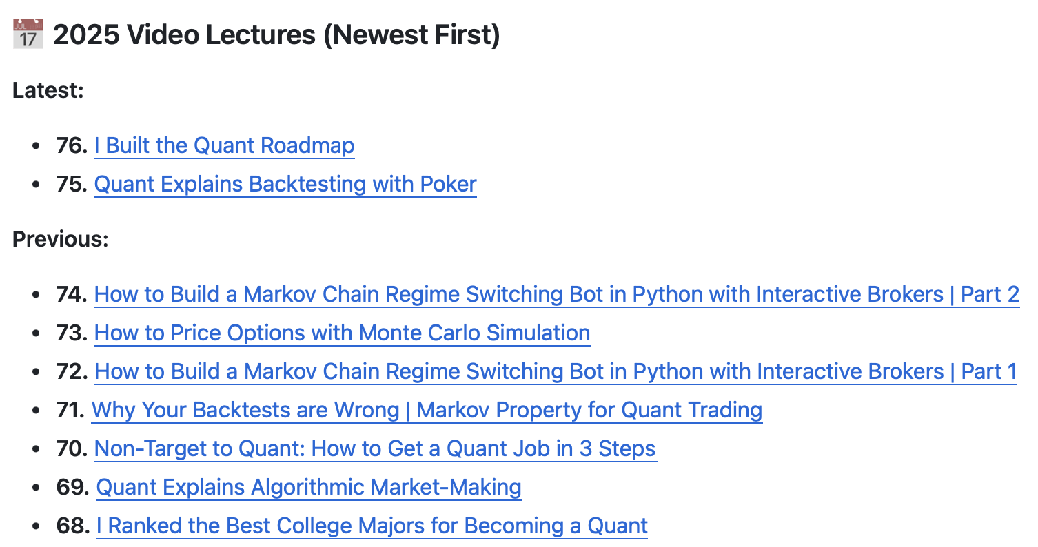 | To say I'm excited for the year ahead would be an understatement. There is so much to look forward to in 2026 including... - 100+ (😳🤠) New Quant Guild YouTube Videos - New and Returning Live Class Sessions - New Quant Guild Features and Courses for Members - Releasing the First of Many Guild Offering in the Bazaar - Growth and Development of a New Social Platform for Quants: discourses.io I want to extend my gratitude for having you (yes, you!) be a part of the Quant Guild community, the support is greatly appreciated and it enables me to continue to develop and share the best quantitative finance knowledge available on the internet. Wishing you a wonderful holiday season and start to the new year! | With that I will leave you to the Weekly Guild Letter. I hope you enjoy, and I hope you learn something! - Roman | | | 🧮 Quant Model of the Week |
| Geometric Brownian Motion |
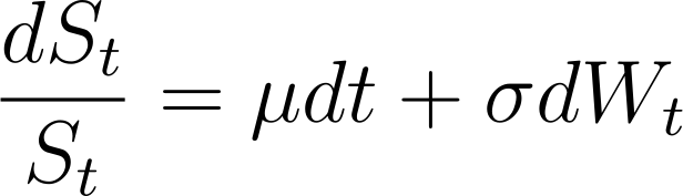
| Some things in markets don’t just wander: they scale. A 1% move means something very different for a $10 stock than for a $1,000 stock, yet both feel “the same” in risk terms. That’s the hallmark of multiplicative behavior: what matters isn’t the dollars, it’s the proportion. Prices grow, shrink, and compound in percentage space, not linear space, and once you see that, it’s obvious that any model pretending otherwise is missing the shape of how markets actually move. Geometric Brownian Motion is the cleanest expression of that idea. Instead of adding noise to the price directly, it lets randomness act on returns, making the entire process scale with itself. The higher the price, the larger the dollar swings, but the volatility stays proportional, a feature that gives you lognormal prices, positive values, and the familiar “compounding effect” built right into the math. It’s simple, almost aggressively so, but it captures something essential: market moves happen in percentages, not points. Here’s what the model looks like: | | | The trick with geometric Brownian motion is that it looks nonlinear and messy in price space, but the moment you take logs, everything straightens out. The multiplicative randomness becomes additive, the curvature disappears, and suddenly you’re staring at an arithmetic Brownian motion, something we already know how to solve cold. | | | That’s the whole punchline, GBM isn’t difficult once you realize it lives a simple life in log space. Solve the linear SDE there, exponentiate, and you recover a process whose paths can grow, compound, and stay positive without any extra heroics. The math feels heavy until you see that one move, and then it’s like, “Oh… that’s it.” | 📈 Model applications Geometric Brownian Motion is the workhorse of quantitative finance, the backbone of Black-Scholes, the simplest nontrivial model where one source of randomness drives the entire asset price. Everything flows from its multiplicative structure: percentage returns stack, compound, and explode or decay exactly the way financial intuition expects them to. Instead of modeling prices additively, GBM says, “returns scale with the level” which is precisely how real assets behave. That’s why Black-Scholes works as cleanly as it does. With a single Brownian driver, the log of the price becomes an arithmetic Brownian motion, which hands you closed-form solutions, tractable hedging, and a complete market. It’s simple, but that simplicity is the reason it became the foundation. And almost every model we use today is really “GBM plus something.”
- Add stochastic volatility? You’re perturbing the diffusion coefficient of GBM.
- Add jumps? You’re bolting a Poisson process onto GBM’s multiplicative engine.
- Add local volatility? You’re letting GBM’s volatility depend on where the process is.
- Add rough volatility? You’re replacing the Brownian motion inside GBM with a rougher signal while keeping the multiplicative frame intact.
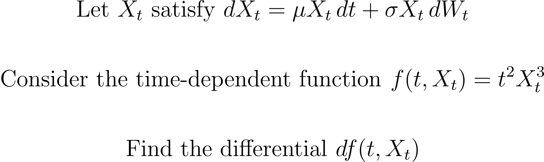
Even interest-rate and credit models borrow the logic, whether they keep or relax the lognormality, the core idea remains: start with GBM’s structure, then layer in the extra physics of markets. GBM is not the end state of modeling; it’s the launchpad. Everything more realistic is just GBM viewed through a more complicated lens. It’s the clean baseline every extension is judged against, the skeleton you keep even when you dress the model in very different clothes. 🎓 A little story When I first learned geometric Brownian motion, it honestly felt like a bit of a cop-out. Everyone kept saying, “Just take the log, solve it as an arithmetic process, then exponentiate back.” And I remember thinking… okay, but how was I supposed to know to do that? It felt like a trick rather than a model, like GBM only worked because someone whispered the magic word: log. But once I understood the deeper idea, it clicked. Arithmetic processes are solvable in closed form. Multiplicative ones usually aren’t. So you don’t fight the multiplicative structure, you transform it into something linear where the math behaves nicely. And once you see that, you see the same move everywhere in quant finance: when something is hard in one domain, switch domains. GBM uses logs. Fourier pricing uses frequency space. Volterra models use integral kernels. Rough vol uses fractional structure. It's the same instinct again and again: don’t wrestle the model where it’s complicated; move it to where it’s simple. And that was the moment GBM stopped feeling like a trick and started feeling like a blueprint. A reminder that half of being a quant is knowing which version of the problem you’re supposed to solve. Logs didn’t cheapen GBM, they revealed it. 💡 Takeaway Markets don’t actually follow geometric Brownian motion, we all learn that pretty quickly once we look at real returns. Volatility isn’t constant, shocks aren’t Gaussian, and sample paths are a lot messier than the clean exponential curves GBM draws. But GBM captures something essential: prices evolve multiplicatively. Returns compound. Percent moves matter more than point moves. And that single structural choice is the backbone of Black–Scholes and a huge amount of the modeling landscape that came after it. Most modern models aren’t replacements for GBM; they’re extensions of it. Stochastic volatility, jumps, local vol, rough vol, stochastic rates, all of them start with the multiplicative structure of GBM and then layer on more realistic dynamics to match the world we actually trade in. GBM gives you the geometry, the positivity, the log-normal intuition, and a clean starting point for risk-neutral pricing. Everything else modifies the volatility, the drift, or the randomness itself. So sure, markets don’t move like GBM. But they move on top of GBM. And that’s the point: it’s the scaffold we build on. The multiplicative structure stays, the realism gets added, and together they give us models that actually help with pricing, hedging, and risk. GBM isn’t the truth, it’s the foundation. | | | 🏆 Quant Question of the Week |
| Solution at the Bottom of this Email 👇 |
| | | Need to study up on topics in math, probability, and finance? 👉 Learn to solve problems like this on Quant Guild — the platform I wish I had when I was studying to become a quant. | | | 📅 Quant Guild Week in Review |
| Backtesting as Poker and the Quant Roadmap |
|
|
|
|---|
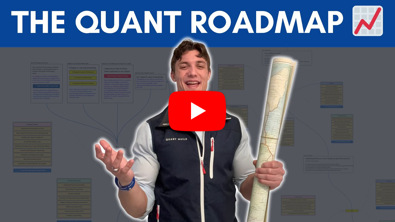
📈 Quant Explains Backtesting with Poker | In this video I use poker to explain what proper backtesting actually looks like and why so many traders get it wrong. I start with a simple analogy: playing pocket aces is just an entry signal. If we simulate hundreds of hands against static opponents who never bluff, never raise, and always continuation bet, pocket aces produce positive expected value. The P/L distribution tilts in our favor, and everything looks great in the backtest. Then I move to the live market version of this idea. When we take that same entry signal into reality, performance collapses because the conditional distribution is completely different from the unconditional one we simulated. In real poker people bluff, raise, trap, and change behavior across regimes. The same is true in trading. One entry signal can behave like a winner in one regime and a loser in another. Treating all occurrences as the same is what breaks most backtests. I show how decomposing expected value into win probability, loss probability, and average win or loss gives us levers to improve a strategy. In the poker example I tighten play by folding when players bet heavily after the flop, which dramatically reduces the average loser. Even though the probability of losing goes up, the losses shrink so much that the strategy returns to positive expectancy. This is exactly what we do in trading when we size up during favorable volatility regimes and hedge or skip entries in hostile ones. The bigger lesson is that every trading signal is conditional. Two signals that look identical on a chart can belong to entirely different distributions depending on volatility, volume, macro climate, sentiment, or any other regime variable. Once you condition correctly and break your strategy into regime specific distributions, your backtests become stable and your live trading results align with your research. Without this, your backtest is wrong by construction. Here's a link to the full video 👇 | | | 🎲 I Built the Quant Roadmap | In this video I walk you through the complete quant roadmap I built to guide anyone from beginner to fully capable quantitative practitioner. I organized every major topic in mathematics, probability and statistics, finance and economics, computer science, and machine learning into levels one, two, and three. The goal is simple. You should always know exactly what to study next, how deep to go in each discipline, and how to measure whether you’ve actually learned the material. I start by explaining how to use the roadmap. You begin at level one and work downward through each discipline in order. I also explain the three stages of learning. First you study the topic. Then you practice it until you can build intuition. Only then can you apply it in the real world. If you cannot apply it, you return to the beginning because you have not actually learned it. I walk through every discipline in detail. In computer science level one you learn the fundamentals and your objective is simple. You should be able to build basic applications from scratch. In mathematics level one you master algebra and geometry so you can set up and solve deterministic problems. In probability and statistics you learn the foundational concepts of distributions, randomness, independence, and conditionality so you can model fixed random variables. In finance and economics you learn the basic theory, but more importantly you learn to think critically because the formal models often fail in the real world. Then I move into level two across all disciplines. You study data structures and algorithms, calculus and linear algebra, probability distributions and inference, the full machine learning development pipeline, and core financial theory. I emphasize that level two is where people finally understand the gap between academic assumptions and the real world. This is where you develop the ability to reason about when models work and when they break. Level three is where everything converges. You study stochastic calculus and PDEs, time series and stochastic processes, advanced machine learning like reinforcement learning and deep sequential models, and high level finance and economics such as risk management, market anomalies, and tail events. At this stage new ideas come from mastery of foundational material. Once you truly understand the basics, you can build your own models, create extensions, and conduct meaningful research. I close the video by reminding you that being a quant is about applying your toolkit to open ended real world problems. You learn, you practice, and you apply. That cycle never stops. The roadmap I made is a living document that expands as the field evolves, and I encourage viewers to comment on anything they think should be added. Here's a link to the full video 👇 | | |
|
|
|---|
|
 | 📈 Why 10,000+ Quants Study on Quant Guild | Quant Guild is the one-stop platform for mastering the math that powers modern finance. With 90+ specialized lessons, adaptive practice with gamified progress that scales with your skill level, real interview questions, courses from A - Z in coding, math, probability & statistics, and exclusive live classes with me, it’s built to take you from fundamentals to the front-office. Everything’s designed for how real quants think and work — focused, practical, and deeply technical. That’s why over 10,000+ students and professionals study on Quant Guild to sharpen their edge and make smarter decisions in the face of uncertainty. |  |
|
|
|---|
| | I'm in QR preparing for technical interviews and your practice helped me brush up on probability, thanks | | |
| | |
|
| | | I learned more here in two days than an entire semester of college | | |
| - Guy on Discord Who DM'd Me |
|
|
|
|---|
|
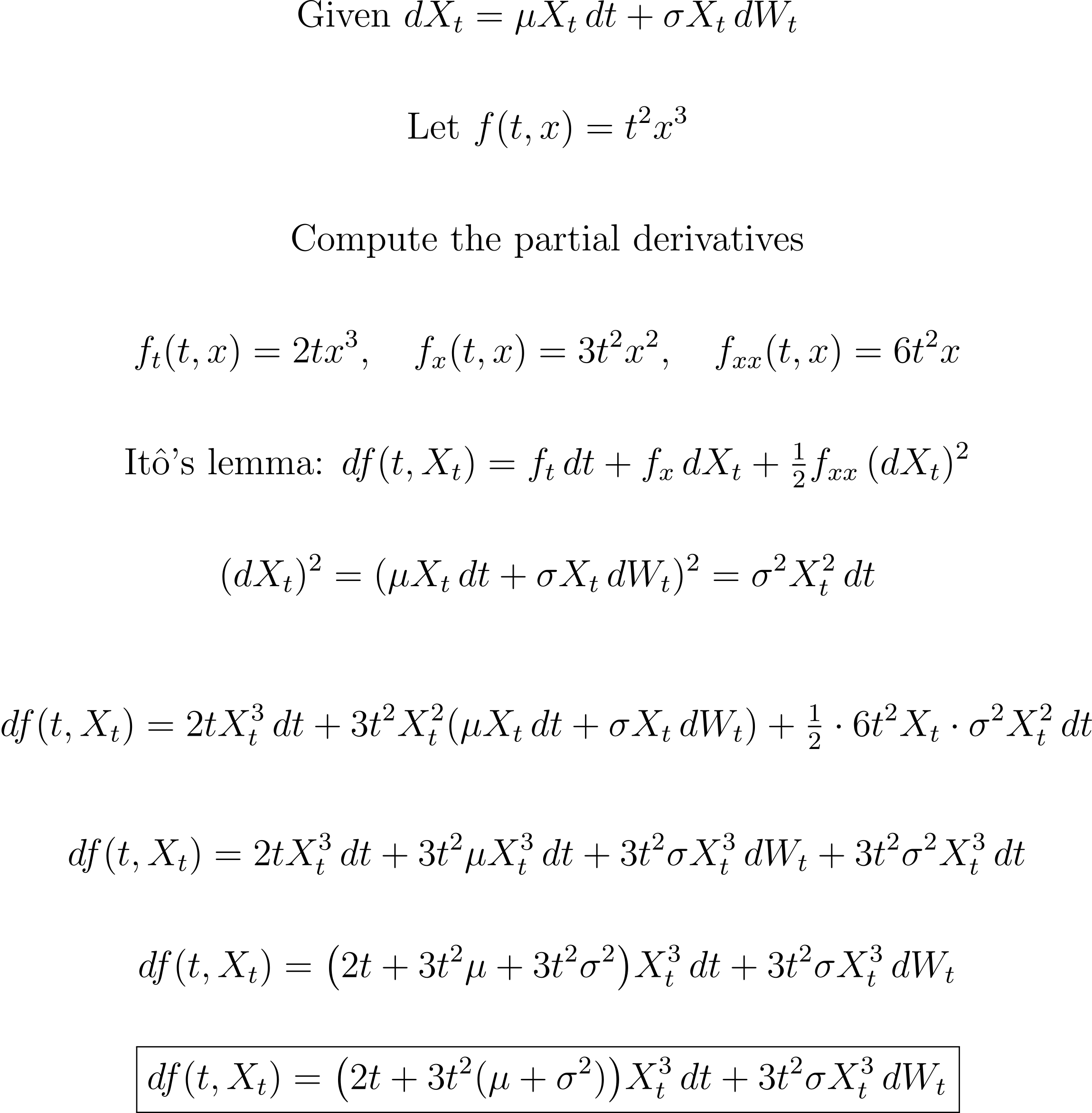
| | ✅ Quant Question of the Week |
| | | | | | |
|
|
|---|
|

 Roman Paolucci