 | | | 📜 A Note from the Guild Leader |
| I'm often asked about the impact of AI in quantitative trading. Large Language Models (LLMs) enable fast ideation and minimum viable products (MVPs), absolutely no doubt about that: quants leveraging artificial intelligence can be 10x more productive. But we suffer the same fate as a calculator, our LLM is really only as smart as our user. If you don't understand how to build what you are intending to (especially in a quant research or trading context) you will be met with an endless series of "You're right! I made a mistake! There is bias in this backtest!" by your LLM. | | | In other words, we don't get something for nothing, this technology is a double edged sword that promotes laziness and unintentional results. This is devastating in the context of scientific trading! If you find yourself asking an AI model "Is this backtest tradable?" or "Is there any bias in this backtest?" I would highly encourage you to read the code yourself and learn the necessary quantitative skills to answer these questions on your own. Don't rely on others (or AI) to make decisions for you, make your own informed decisions fully understanding the implications and limitations of your models and assumptions. | With that I will leave you to the Weekly Guild Letter. I hope you enjoy, and I hope you learn something! - Roman | | | 🧮 Quant Model of the Week |
| Correlated Brownian Motions |
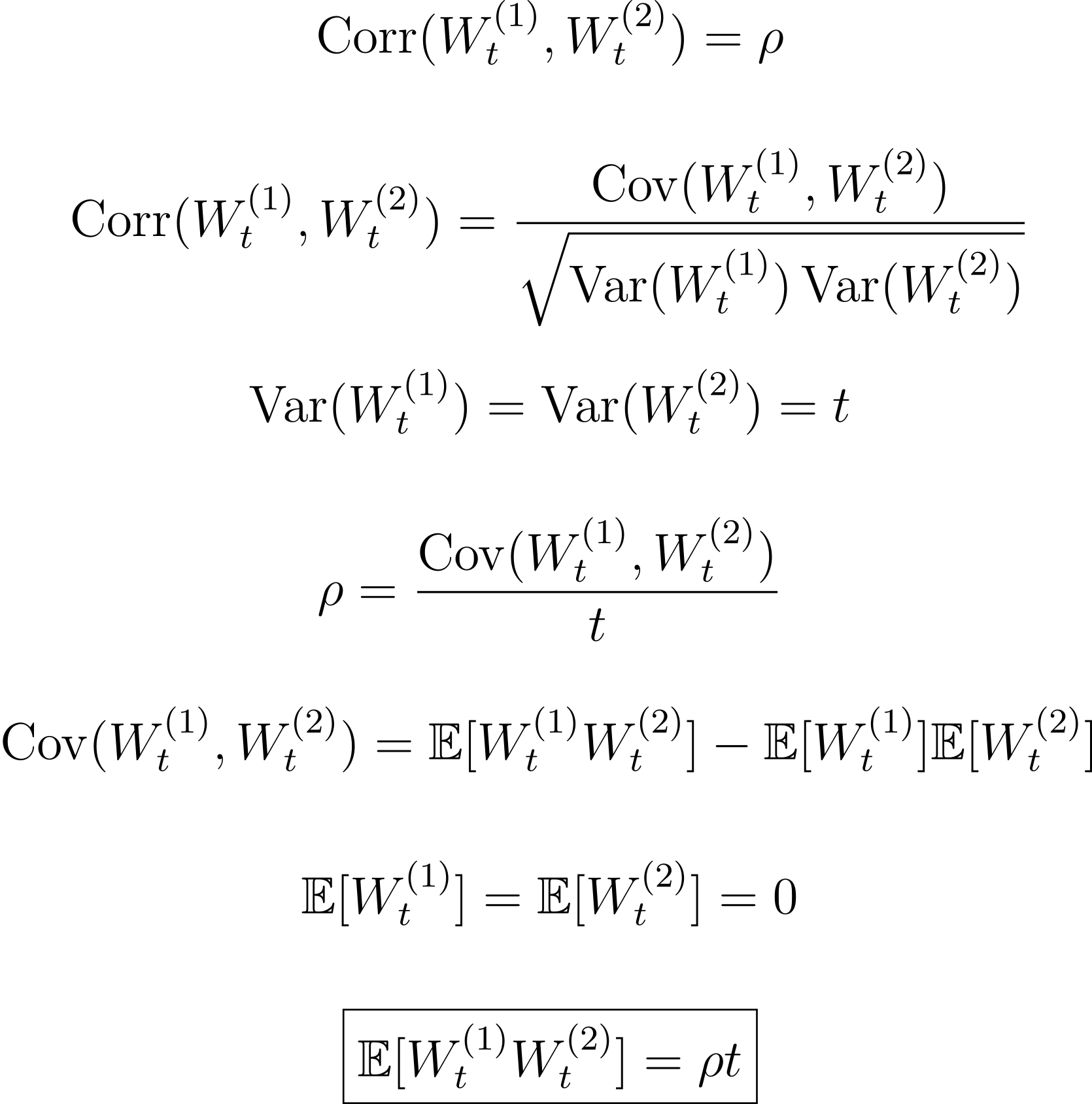
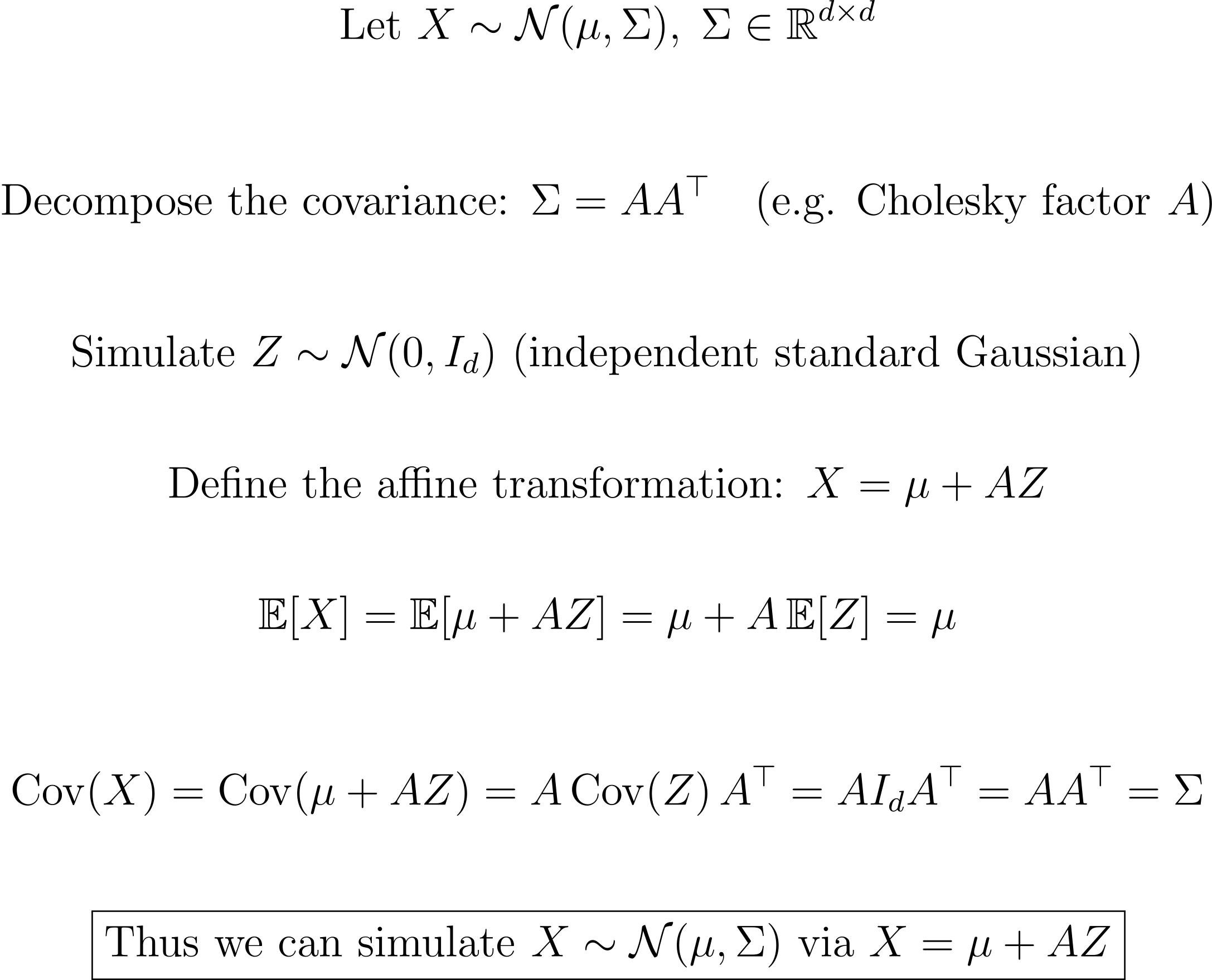
| Markets rarely move one asset at a time. News doesn’t hit a single ticker; it washes across sectors, curves, regions, and asset classes all at once. A surprise rate print shifts currencies, credit, equities, vol surfaces - you name it. Even on quiet days, assets tend to breathe in sync, nudged by the same flows and the same macro undercurrents. The idea that every asset has its own private randomness just doesn’t survive first contact with real data. Correlated Brownian motions give us the simplest mathematical language for this shared uncertainty. Instead of imagining each asset being jostled by its own independent noise, we let them share a portion of the same shock. One part idiosyncratic, one part systemic. Turn the correlation up and their paths start to echo each other; turn it down and they drift apart. It’s a small adjustment in the model, but it encodes something foundational about markets: assets don’t just move, they move together. Here’s what the correlation structure looks like for standard Brownian motions: | | | That's just the formal way of saying "these Brownian motions move together on average with a correlation of rho". So if that's what it looks like formally to exhibit a covariance (correlation) structure, how do we actually generate it? There are many different ways to go about this but the most intuitive comes from decomposing the covariance matrix and then simulating a standard Gaussian. This seems overly complicated at first but observe how decomposing the desired covariance matrix yields something we can multiply with our standard Gaussian (which is easy to simulate). Then if we take the covariance (correlation) of that product we have mechanically induced the desired structure. | | | That's the how and why behind correlated Brownian motions. We can decompose the desired covariance matrix and use it in the affine transformation of a standard normal gaussian draw to produce the desired correlation structure. | 📈 Model applications Correlated Brownian motions are one of those building blocks in quantitative finance that seem almost too simple, until you try modeling anything with more than one asset and suddenly you can’t live without them. They’re the backbone of multi-asset pricing, the foundation of portfolio risk models, and the cleanest way to let different sources of uncertainty talk to each other. Markets don’t move in isolation, and SDEs with correlated Brownian drivers are how we encode that. Once you introduce correlation into your diffusion terms, whole classes of models open up. Portfolio variance becomes something you can actually compute; co-movement becomes something you can express cleanly instead of hand-waving away. Anything involving joint distributions from equity-credit hybrids, FX-equity triangles, to multi-curve rate models starts with a vector of Brownian motions tied together through a correlation matrix. Even the leverage effect in equity models, a negative relationship between price moves and volatility, can be captured by correlating the Brownian motion driving the asset with the one driving its volatility. Suddenly a simple diffusion system behaves like real markets: volatility kicks up after drops, calms after rallies, and the whole system breathes as one. And this is just the beginning. Correlated Brownian motions underpin: stochastic volatility models, where price and volatility shocks must interact Heston-style dynamics, where correlation shapes the skew multi-factor interest rate models, where curves move in locked patterns basket and spread options, where payoff depends on joint behavior credit-equity models, where distress bleeds across markets
It’s not that correlated Brownian motions are the final word: they’re the starting word. Most realistic multi-asset or multi-factor models are “correlated Brownian motion plus structure.” Add jumps, add stochastic vol, add roughness, add regimes… the dependence between the drivers always sits at the core. Correlated Brownian motions aren’t just a modeling choice; they’re the mathematical expression of something every trader already knows: assets are connected. Their risks are shared. Their randomness is intertwined. And without this structure, none of our pricing, hedging, or risk frameworks would describe markets even remotely well. 🎓 A little story The first time I really understood correlated Brownian motions, it wasn’t from a textbook definition or a proof, it was from actually trying to simulate them. Up to that point, “correlation” felt like this mysterious knob you turned in a model, and somehow two processes magically started moving together. It didn’t feel mechanical or grounded; it felt like declaring a relationship and hoping the math saluted. Then I learned about decomposition. You take the covariance matrix you want, break it apart with something like a Cholesky or spectral factorization, and suddenly the whole thing becomes concrete. You feed independent Brownian motions through that transformation and — BOOM — the output must have the correlation structure you prescribed. Not because of hope or intuition, but because linear algebra says so. In the ensemble average sense, the simulation is guaranteed to reflect the covariance you built into it. And that was the moment it clicked for me. Correlated Brownian motions aren’t “mysterious” at all. They’re engineered. You literally build the dependence you want, plug in the randomness, and watch the system behave exactly the way the covariance matrix says it should. Once you see that, you start noticing the pattern across quant finance: half of modeling is specifying the structure you need, and the other half is choosing the right transformation to make randomness obey that structure. It stopped feeling like magic and started feeling like machinery, clean, controlled, and deeply satisfying. Correlation isn’t a vibe; it’s a construction. 💡 Takeaway If our models don’t take correlations seriously, we’re building frameworks that are more wrong than they need to be. Markets don’t move one asset at a time; they move in clusters, waves, and shocks that ripple across instruments. Correlation is the wiring behind that behavior. Leave it out, and your pricing, hedging, and risk estimates start drifting away from reality before you even run the first simulation. Most modern multi-asset models aren’t inventions from scratch, they’re “correlated Brownian motion plus structure.” Add stochastic volatility and you get skew. Add jumps and you get crisis behavior. Add dynamic correlation and you start capturing what we actually see in markets: dependence that tightens in stress, loosens in calm, and shifts with macro regimes. The correlation matrix isn’t a static input; it’s a living object, one that often moves faster than the prices themselves. So no, markets don’t follow simple correlated diffusions any more than they follow geometric Brownian motion. But these correlated drivers give us the scaffold. They capture the shared randomness, the co-movement, the systemic component of risk, the part that actually matters when the world gets loud. Improve the correlation structure and everything downstream improves with it: portfolio risk, derivative pricing, hedging, scenario generation, all of it. Correlation isn’t a detail. It’s the structure underneath the surface. And the closer we get that structure to reality, even with time-varying, state-dependent, or regime-shifting dependence, the more useful and honest our models become. | | | 🏆 Quant Question of the Week |
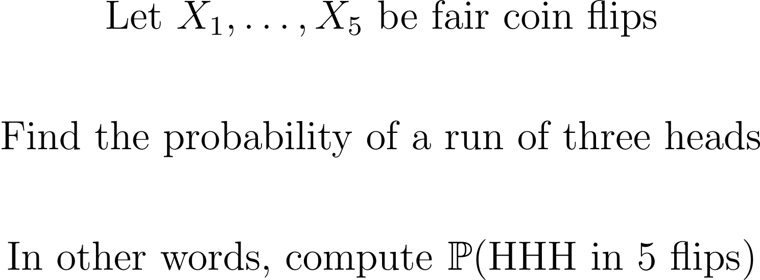
| Solution at the Bottom of this Email 👇 |
| | | Need to study up on topics in math, probability, and finance? 👉 Learn to solve problems like this on Quant Guild — the platform I wish I had when I was studying to become a quant. | | | 📅 Quant Guild Week in Review |
| Profitable vs Tradable and Alpha vs Beta |
|
|
|
|---|
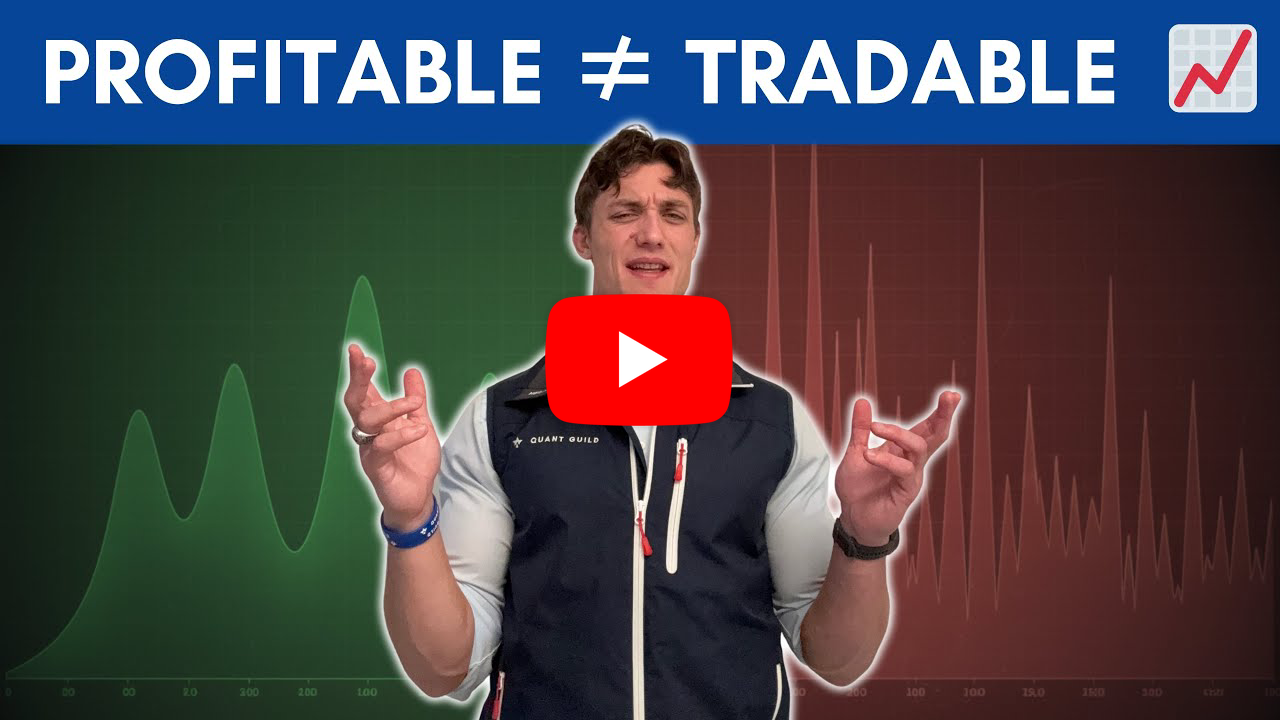
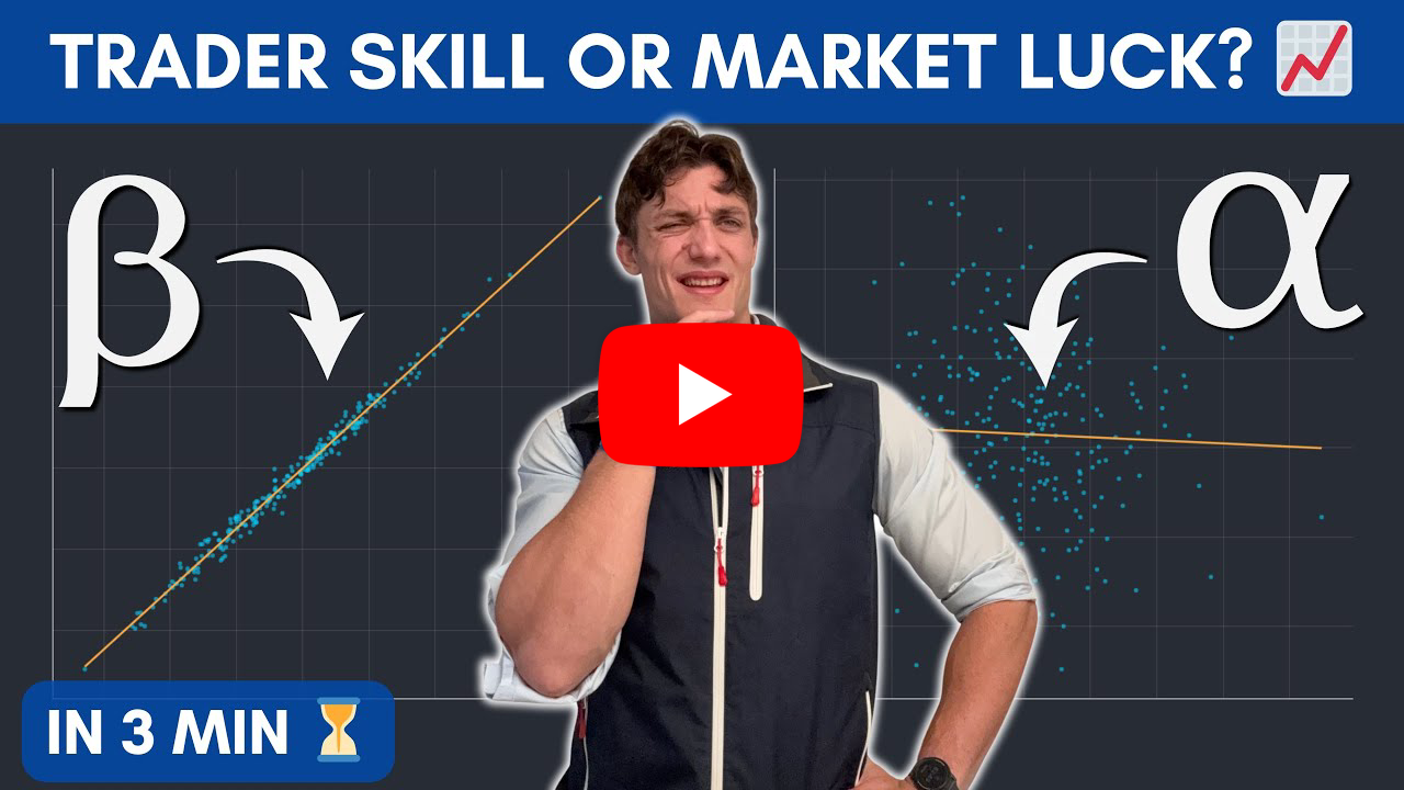
📈 Profitable vs Tradable: Why Most Strategies Fail Live | In this video I explain one of the biggest misconceptions in trading: asking whether someone is “profitable” is the wrong question. Profitability is backward looking. What actually matters is whether a strategy is tradable in a forward looking capacity. Both discretionary and quantitative traders profit from the exact same statistical mechanism. They accumulate wealth only if the underlying P and L distributions remain stable across time. That stability is what most strategies completely lack, which is why they collapse the moment they go live. I start by defining what an edge actually is. An edge is nothing more than positive expected value, which we can fully decompose into the probability of winning, the probability of losing, the average winner, and the average loser. This decomposition gives us two distributions. A distribution for winners and a distribution for losers. If those distributions remain stable across sample periods, then the strategy is tradable. If they do not, the backtest is meaningless. I walk through a real example using Nvidia from 2020 to 2023 and then compare the results to 2024 through 2025. The backtest shows a clean, profitable strategy with a stable expectancy. When traded live, the distributions completely fall apart. The win rate stays roughly the same, but the average winner and loser change dramatically because the distributions themselves change shape. That shift is what destroys expectancy and reveals that the strategy was never tradable. From there I show how stability comes from structure. You need economically or statistically meaningful signal generation, not brute force backtesting. I demonstrate this using volatility regimes created from quadratic variation. By conditioning on low, mid, and high volatility states, we can see that the same entry signal produces fundamentally different P and L distributions in each regime. But because the regime classification is unstable in the low and high buckets, only the mid-volatility regime displays stability both in sample and out of sample. That stability upstream in the regime is what creates stability downstream in the P and L. I emphasize that this is a data science problem. Everyone wants to train models and look at Sharpe ratios, but the real work is in correctly modeling regimes, validating feature stability, and ensuring that the distributions feeding your strategy are not drifting uncontrollably. Without that, machine learning models, hidden Markov models, and even simple rule based strategies will all fail live. The big takeaway is simple. A profitable backtest means nothing. A tradable strategy requires stable distributions across time. If you can build structure that induces that stability, you have something real. If you cannot, the strategy is doomed the moment you take it live. Here's a link to the full video 👇 | | | 🎲 Trader Skill or Market Luck? Alpha vs Beta in 3 Min | In this video I break down what alpha actually is by comparing two hedge fund portfolios that appear identical on the surface. Both produce Sharpe ratios around two and a half, which would normally suggest that both managers are doing an equally strong job. But Sharpe alone cannot tell us where that performance is coming from. To separate true trading skill from simple market exposure, I turn to the capital asset pricing model and show how we can regress portfolio returns against market returns to uncover beta and alpha. I simulate two hedge fund portfolios and walk through the regression results. The first fund shows a very strong correlation with the market, meaning most of its return is driven by beta. The second fund shows almost no correlation at all. When we decompose their returns, the first portfolio is revealed to be almost entirely market driven, while the second is one hundred percent alpha. The performance may look similar in a bull market, but they could not be more different in a bear market. One collapses with the market, while the other continues to generate value because its performance comes from genuine structural inefficiency rather than market drift. The key idea is simple. Alpha is forward looking. It tells us whether a portfolio’s performance is due to actual skill and edge rather than luck or exposure. Two strategies can produce the same Sharpe ratio, but only one will survive when market conditions change. That is the difference between luck and skill, and that is what makes alpha such a powerful metric. Here's a link to the full video 👇 | | |
|
|
|---|
|
 | 📈 Why 10,000+ Quants Study on Quant Guild | Quant Guild is the one-stop platform for mastering the math that powers modern finance. With 90+ specialized lessons, adaptive practice with gamified progress that scales with your skill level, real interview questions, courses from A - Z in coding, math, probability & statistics, and exclusive live classes with me, it’s built to take you from fundamentals to the front-office. Everything’s designed for how real quants think and work — focused, practical, and deeply technical. That’s why over 10,000+ students and professionals study on Quant Guild to sharpen their edge and make smarter decisions in the face of uncertainty. |  |
|
|
|---|
| | I'm in QR preparing for technical interviews and your practice helped me brush up on probability, thanks | | |
| | |
|
| | | I learned more here in two days than an entire semester of college | | |
| - Guy on Discord Who DM'd Me |
|
|
|
|---|
|
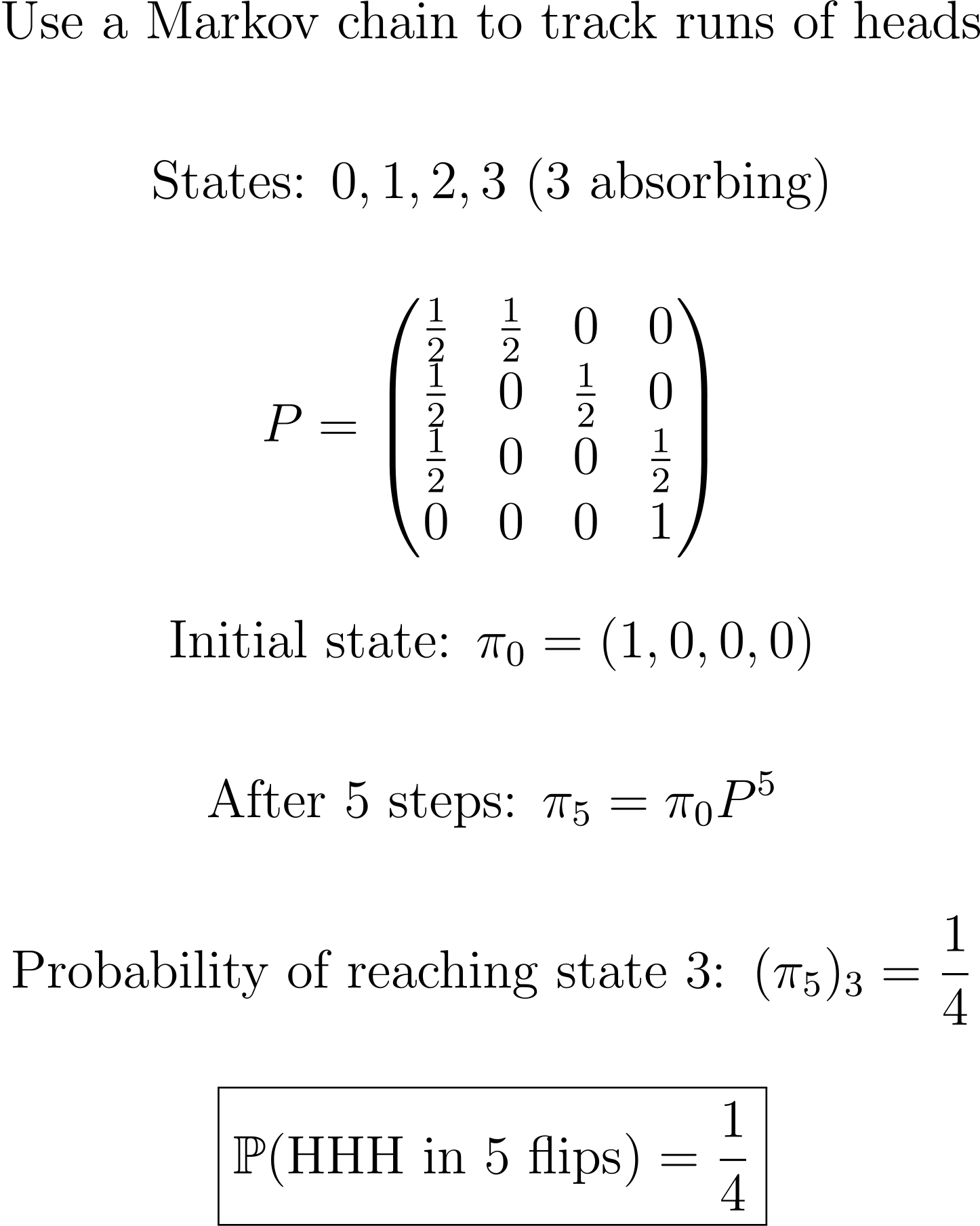
| | ✅ Quant Question of the Week |
| | | | | | |
|
|
|---|
|

 Roman Paolucci