 | | | 📜 A Note from the Guild Leader |
| What is the difference between a portfolio manager or trader with effective timing of exposure to priced risk and a structural inefficient? Is timing exposure (beta) really alpha? In other words, if I know when to increase or decrease my market exposure and I can capitalize on reversion and momentum of that factor is that a strategy that produces alpha? Shouldn't alpha be orthogonal to facets of priced risk? | | | In the CAPM framework, alpha is the constant return from stock-picking skill, while timing exposure is the variable return from shifting beta (market sensitivity) based on forecasts. Using extensions like Treynor-Mazuy or Henriksson-Merton, timing appears as convexity, a "kinked" or "curved" line showing higher exposure in bull markets and lower exposure in bear markets. If this shift is discretionary, it’s labeled alpha; if it follows a fixed rule, it is classified as smart beta. The difference matters more than you might think. Smart beta strategies and strategies that produce alpha (trade a structural inefficiency) produce different risks when capital is allocated. Alpha can be crowded out, smart beta strategies may observe severe reversion or structural breaks making the selection criteria for exposure obsolete in producing returns where alpha would continue to perform as it is likely orthogonal to that break by definition of the exposure. Both are effective, the choice in which to trade comes down to availability and of course timing! | With that I will leave you to the Weekly Guild Letter. I hope you enjoy, and I hope you learn something! - Roman | | | 🧮 Quant Model of the Week |
| Autoregressive Model - AR(p) |
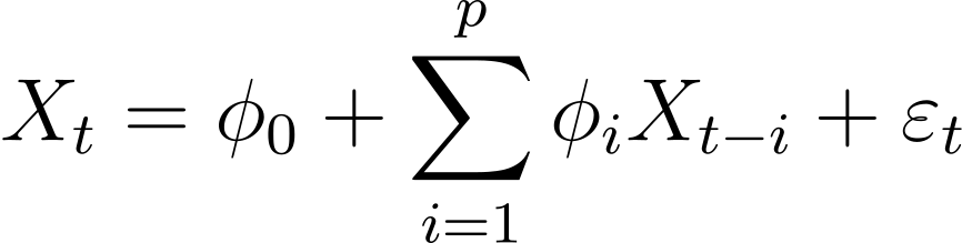
| Signals strengthen, decay, and occasionally resurrect themselves months later. Markets don’t reset after every tick, today’s value leans on yesterday’s, which leaned on the day before that. The idea that each observation is completely fresh just doesn’t survive first contact with a time series. Autoregressive (AR) processes are the simplest mathematical way to express that temporal dependence. Instead of treating each data point as independent noise, an AR model lets the past feed directly into the present. A shock doesn’t vanish when it arrives; it echoes forward, gradually fading (if the process is stationary) or compounding into something unstable (if it isn’t). Turn the AR coefficient down and shocks dissipate quickly; turn it up and the series holds onto memory, trending or drifting depending on the regime. It’s a tiny adjustment — “today depends on yesterday” — but it captures something foundational about markets: time leaves fingerprints. And whether a process is stationary or non-stationary determines whether those fingerprints fade or accumulate, whether the series stabilizes around a mean or wanders off indefinitely. Here’s what the AR structure looks like: | | | The AR(p) model says that the value of a process at time t is essentially a weighted blend of its own past. Each coefficient tells you how strongly a previous observation pushes on the present, while the constant sets the baseline level the series tends to orbit. The only genuinely “new” information is the shock term, which injects randomness but then propagates forward through the autoregressive structure. Depending on the size and arrangement of the coefficients, the process can quickly forget its past or cling to it, producing anything from stable, mean-reverting behavior to persistent, drifting dynamics. In one line, the model captures the basic truth of time series: today is never independent of yesterday. | 📈 Model applications Autoregressive processes are one of the first tools quants reach for when dealing with time-series data, and for good reason: they’re simple, interpretable, and capture the essential idea that markets don’t reset each period, they carry momentum, drift, and the lingering effects of past shocks. An AR model says “today depends on yesterday,” and that alone gets you surprisingly far. You can model persistence in returns, decay in signals, mean reversion in spreads, or the slow bleed of an alpha that’s losing its edge. Stationary AR models fade their memory and stabilize; non-stationary ones accumulate history and wander. Both behaviors show up constantly in financial data. But the real power of AR processes isn’t that they’re perfect, it’s that they’re honest about how imperfect time series really are. They remind you that structure only holds until it doesn’t. Parameters drift. Regimes break. A beautifully stationary AR(1) can look great for five years, then completely fall apart the moment volatility shifts or macro conditions change. Markets are always evolving, and an AR model can only track that evolution for as long as the underlying behavior stays remotely stable. Still, AR processes sit at the core of almost everything more sophisticated. Add noise with memory and you’re walking toward ARMA and ARIMA. Add conditional volatility and you land on ARCH and GARCH. Add multivariate structure and you get VARs for macroeconomic dynamics. Add state-switching and you’re in Markov regime models. The point is the same: AR dynamics are the backbone of time-series modeling, the simplest description of how the past echoes into the present, and the scaffolding on which more realistic ideas are built. And yet, no matter how intricate the model becomes, the lesson remains: a time series reflects real behavior. It’s shaped by regimes, market cycles, liquidity conditions, and human decisions. There’s only so much structure you can impose before reality snaps it. AR models work until the world changes, and the world is always changing. 🎓 A little story The first time I took a time-series class, this was in high school at a local college, long before I knew what a stochastic process even was, we learned about non-stationarity, homoskedasticity vs. heteroskedasticity, unit roots, all that stuff. And my honest reaction was: what is the point? If nothing is constant, if the variance changes, if the “rules” break every few months, why are we modeling any of this? It felt like building a house on sand. Every example came with a disclaimer: “only valid if the process is stationary,” “only stable under certain assumptions,” “sensitive to structural breaks.” Great. So… what am I supposed to do with that? It wasn’t until much later that I understood the real purpose. We don’t build AR models because we believe the world is stationary, we build them because they help us understand how a system behaves when it’s not. The point isn’t to pretend regimes don’t change; it’s to identify when they have changed. We don’t rely on a single AR equation to predict the future; we use it alongside volatility models, regime detectors, structural indicators, and stress scenarios to map out the landscape of possible outcomes. Modeling isn’t about declaring certainty, it’s about preparing for uncertainty. Once that clicked, AR processes stopped feeling naive and started feeling like tools: imperfect on their own, but powerful when combined with an understanding that markets break, adapt, shift, and evolve. In practice, you’re not trying to predict the exact path; you’re assessing likelihoods, spotting instability, and building intuition for when the underlying regime is quietly changing underneath your feet. Models don’t give you the full truth, they give you the structure you need to make informed decisions in a world where very little stays constant. 💡 Takeaway If our models don’t take temporal dependence seriously, we end up building time-series frameworks that are more wrong than they need to be. Markets don’t generate data as a sequence of unrelated points; they evolve through habits, shocks, drifts, and regimes that bleed into one another. Autoregressive processes are the wiring behind that behavior. Ignore lag structure, and your forecasts, signals, and risk estimates drift away from reality before you even begin. Most time-series models aren’t invented from scratch, they’re “AR(p) plus structure.” Add moving averages and you capture smoother dynamics. Add conditional volatility and you start modeling clustered risk. Add integration and you get trending, unit-root behavior. Add regime-switching and you recover the sudden breaks and macro shifts that show up everywhere in real data. An AR model isn’t the full picture; it’s the scaffolding we build richer dynamics on top of. So no, markets don’t follow clean, stationary AR processes any more than they follow perfect diffusions. But AR structure still gives us the backbone: the persistence, the decay, the memory, the parts that matter when we’re trying to understand how shocks propagate through time. Improve that structure with time-varying parameters, state changes, or volatility dynamics, and everything downstream improves with it: forecasting, signal design, risk modeling, scenario generation. Autoregression isn’t a detail. It’s the temporal architecture underneath the surface. And the closer our models come to reflecting the true, shifting nature of markets, whether stationary for a while, drifting for a while, or breaking altogether, the more honest and useful our quantitative tools become. | | | 🏆 Quant Question of the Week |
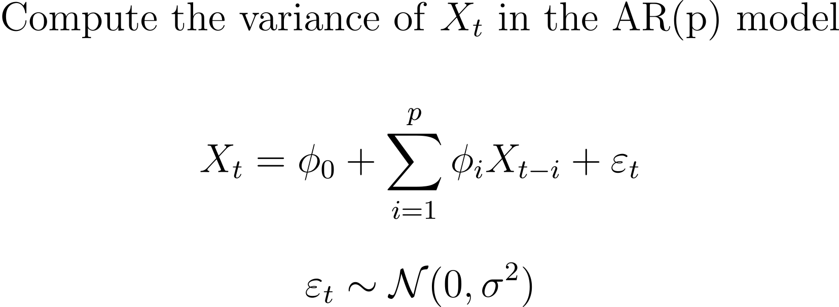
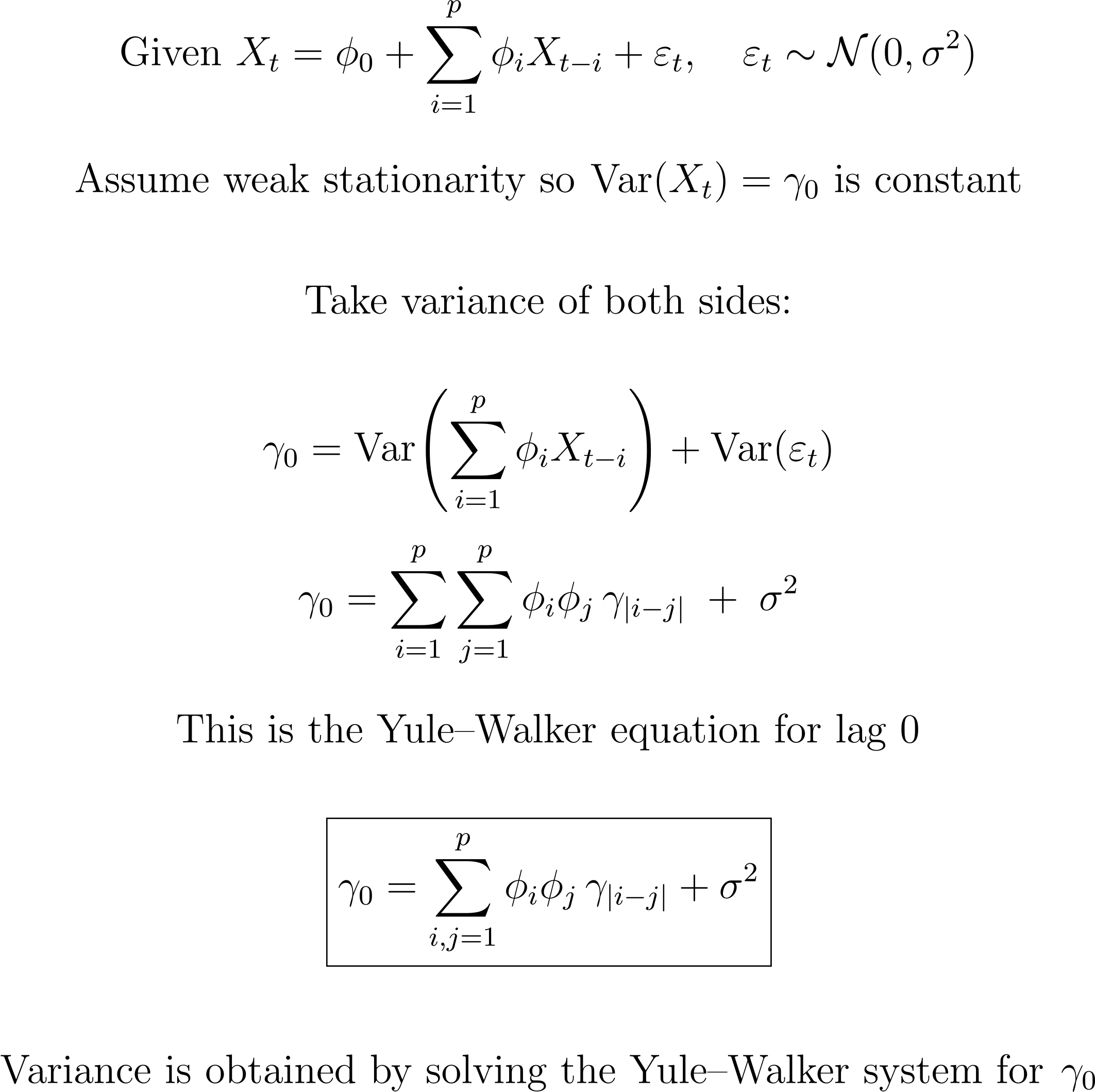
| Solution at the Bottom of this Email 👇 |
| | | Need to study up on topics in math, probability, and finance? 👉 Learn to solve problems like this on Quant Guild — the platform I wish I had when I was studying to become a quant. | | | 📅 Quant Guild Week in Review |
| Quant Interviews and Top 5 Quant Papers |
|
|
|
|---|
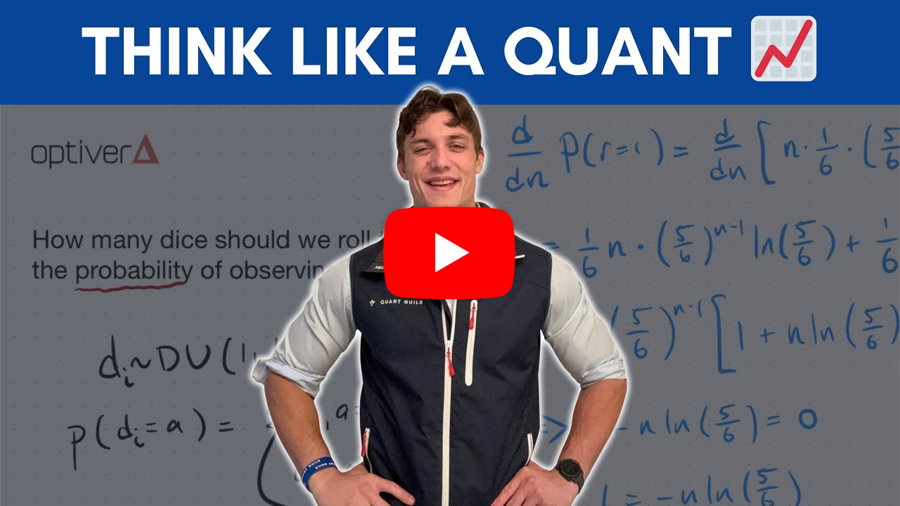
📈 My Approach to Solving Quant Interview Questions | In this video I walk through exactly how I approach quant interview questions from start to finish. Instead of memorizing tricks or canned solutions, I show you how to think like a quant: identify key words, translate the problem into familiar probability structures, and connect every step back to foundational topics in math, statistics, and probability. The example I use is a real Optiver question: How many dice should you roll to maximize the probability of observing exactly one six? I start by showing why you should never jump straight into general cases. Begin with what you know. For a single fair die, the probability of rolling a six is one sixth. From there, rather than getting tangled in messy “or” statements, I reduce the problem to a success–failure framework. Rolling exactly one six is a Bernoulli success, so multiple dice become multiple Bernoulli trials. That translation immediately reveals the correct tool: the binomial distribution, which tells us the probability of observing exactly one success in n trials. Once the problem is reframed, the interview becomes a simple optimization task. I derive the probability function, take its derivative with respect to n, and find the critical point at approximately 5.48. Because the number of dice must be an integer, we check the surrounding values, five and six, and find that both yield the same maximum probability. The bigger lesson is that quant interview questions almost always collapse into familiar structures once you express them correctly. If you understand your probabilistic toolkit deeply, you never need to memorize solutions. You just translate, simplify, and solve. Here's a link to the full video 👇 | | | 🎲 Top 5 Papers that Built Modern Quant Finance | In this video I walk through the five research papers that shaped the entire field of quantitative finance. These papers form the backbone of everything we do today in pricing, risk, portfolio theory, and computational modeling. I start with Louis Bachelier’s 1900 dissertation, the forgotten thesis that introduced Brownian motion and the first mathematical model of option pricing decades before Einstein formalized the physics. He essentially built financial mathematics out of thin air, long before the rest of the world was ready for it. Next I cover the development of portfolio theory and the capital asset pricing model. Markowitz introduced diversification as the only free lunch, and Sharpe extended that work to show that only systematic risk should be rewarded. This is where beta and alpha are born, and where the modern factor model ecosystem begins. I show simulations that illustrate the difference between pure beta exposure and true alpha, reinforcing why this framework is still central to how quants evaluate performance today. From there I move into the seismic shift brought by Black and Scholes in 1973. Their replication argument changed the world by showing that in a complete, frictionless market with one source of randomness, the price of an option must equal the cost of continuously hedging it. This gave us the Black–Scholes equation, implied volatility, and a systematic way to price derivatives. Decades later, Feynman–Kac would unintentionally confirm their result by proving that the PDE solution and the risk-neutral expectation must match. I then explain how the crash of 1987 revealed that constant volatility assumptions were violently wrong. This led to Dupire’s local volatility model, which uses the volatility surface itself as a function of strike and maturity. Local vol allows you to calibrate to liquid instruments and then price exotics in a consistent way. It is the simplest extension of Black–Scholes that fixes one of its biggest real-world failures. Finally, I highlight one of my favorite papers in the entire literature: Carr and Madan (1999) and their Fourier transform method for option pricing. If you know the characteristic function of the underlying process, you can transform the problem, solve it instantly, and invert it back. It bypasses slow simulation entirely and opened the door to modern calibration techniques, stochastic volatility models, and eventually neural network approximators for pricing. The video ends with an executive summary tying all five works together and a preview of upcoming topics like Kalman filters, non-Markovian models, Poisson processes, rough volatility, and new quant builds. These papers are the reason the field looks the way it does today, and understanding them gives you the “why” behind everything quants study and build. Here's a link to the full video 👇 | | |
|
|
|---|
|
 | 📈 Why 10,000+ Quants Study on Quant Guild | Quant Guild is the one-stop platform for mastering the math that powers modern finance. With 90+ specialized lessons, adaptive practice with gamified progress that scales with your skill level, real interview questions, courses from A - Z in coding, math, probability & statistics, and exclusive live classes with me, it’s built to take you from fundamentals to the front-office. Everything’s designed for how real quants think and work — focused, practical, and deeply technical. That’s why over 10,000+ students and professionals study on Quant Guild to sharpen their edge and make smarter decisions in the face of uncertainty. |  |
|
|
|---|
| | I'm in QR preparing for technical interviews and your practice helped me brush up on probability, thanks | | |
| | |
|
| | | I learned more here in two days than an entire semester of college | | |
| - Guy on Discord Who DM'd Me |
|
|
|
|---|
|
| | ✅ Quant Question of the Week |
| | | | | | |
|
|
|---|
|

 Roman Paolucci