📜 A Note from the Guild Leader |
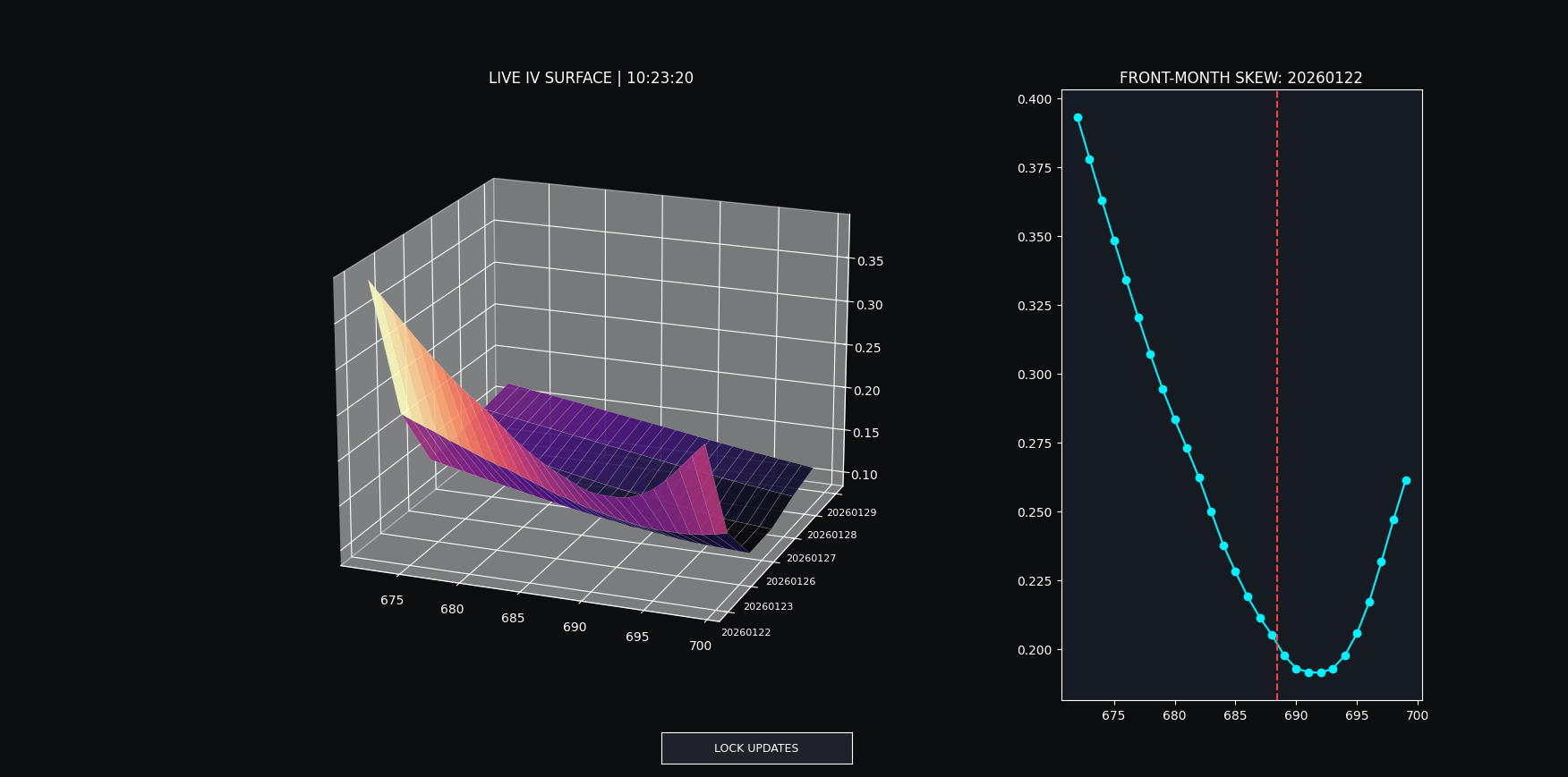
I want to share a note on what I consider to be the most important scientific construct in the trading of financial derivatives: the implied volatility surface. What does it tell us, how is it useful, and how can we access this information in a structured (and algorithmic) way as retailers? |
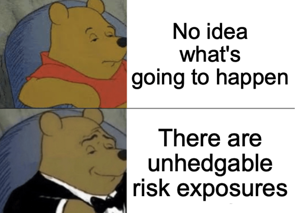
The volatility surface isn't just about "Black-Scholes" and the idea that their model implies a flat surface. As a matter of fact, that is a feature of their framework, not a bug. We can select a set of option contracts for a series of strikes (moneyness) and maturities (time to expiration) and observe the way traders demand to be compensated for unhedgable risk relative to the instrument being traded. This not only explains the lack of symmetry across the skew but it also enables the market to provide pricing for these unhedgable risks in equilibrium, enabling market-makers to extrapolate prices for more exotic instruments consistent with the market's forward outlook on these exposures. |
 |
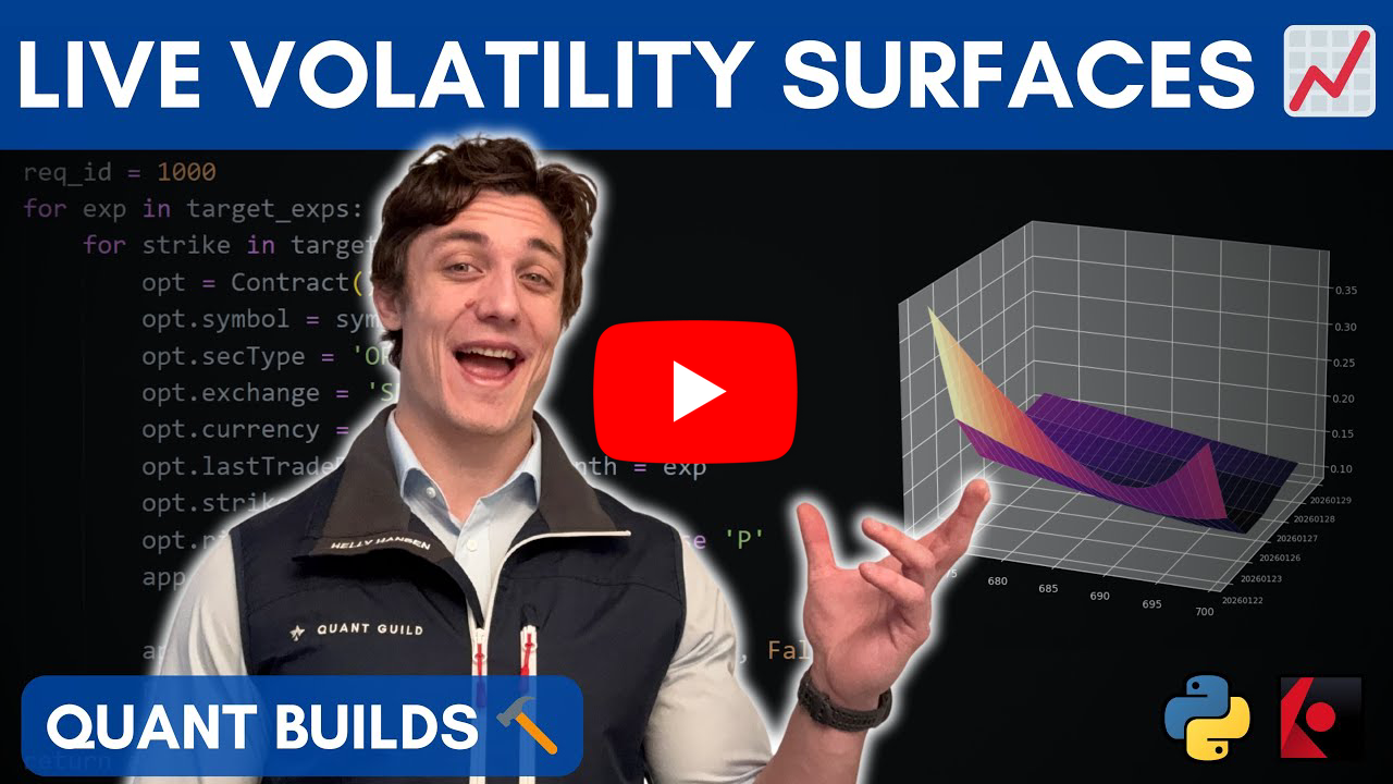
Institutional clients of Bloomberg have easy access to these surfaces for a particular underlying via the OVDV command, but how can retailers find this information? Well last week I created one of the most important videos my channel will ever produce: How to Build a Live Volatility Surface in Python (Interactive Brokers); showing everyone how to construct this object for model calibration, extrapolation, and of course, trading. |
With that I will leave you to the Weekly Guild Letter. I hope you enjoy, and I hope you learn something! - Roman |
🧮 Quant Model of the Week |
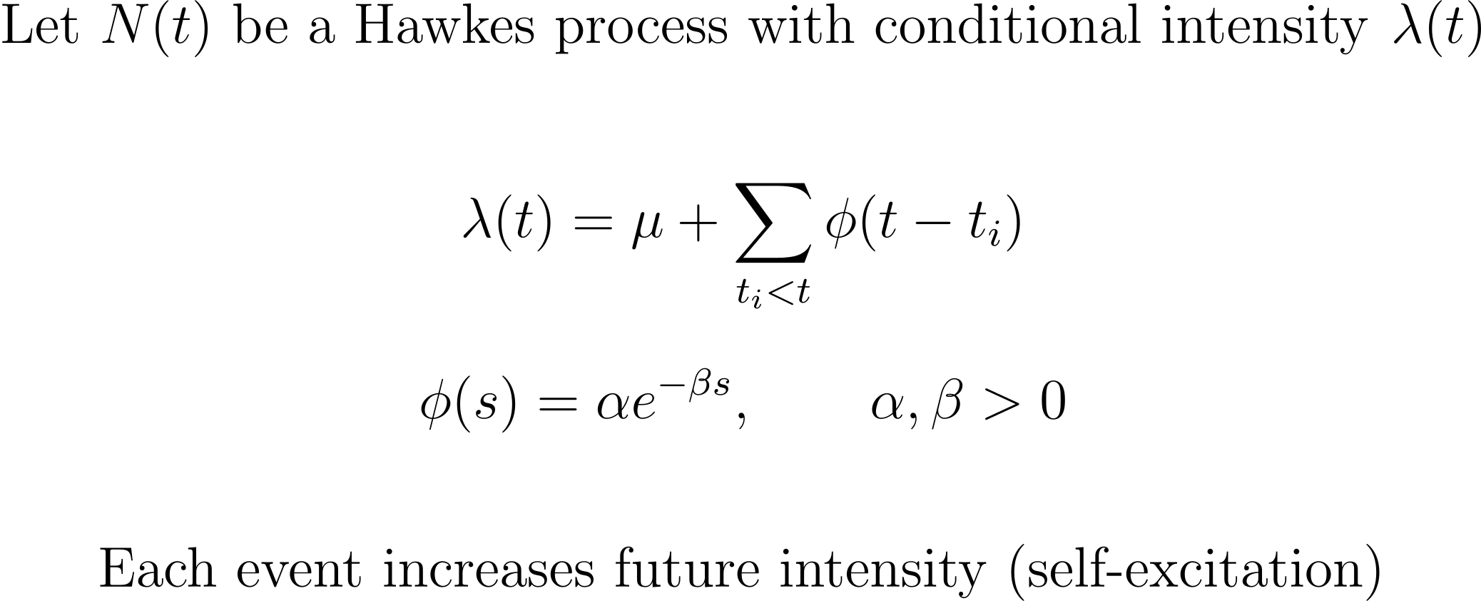
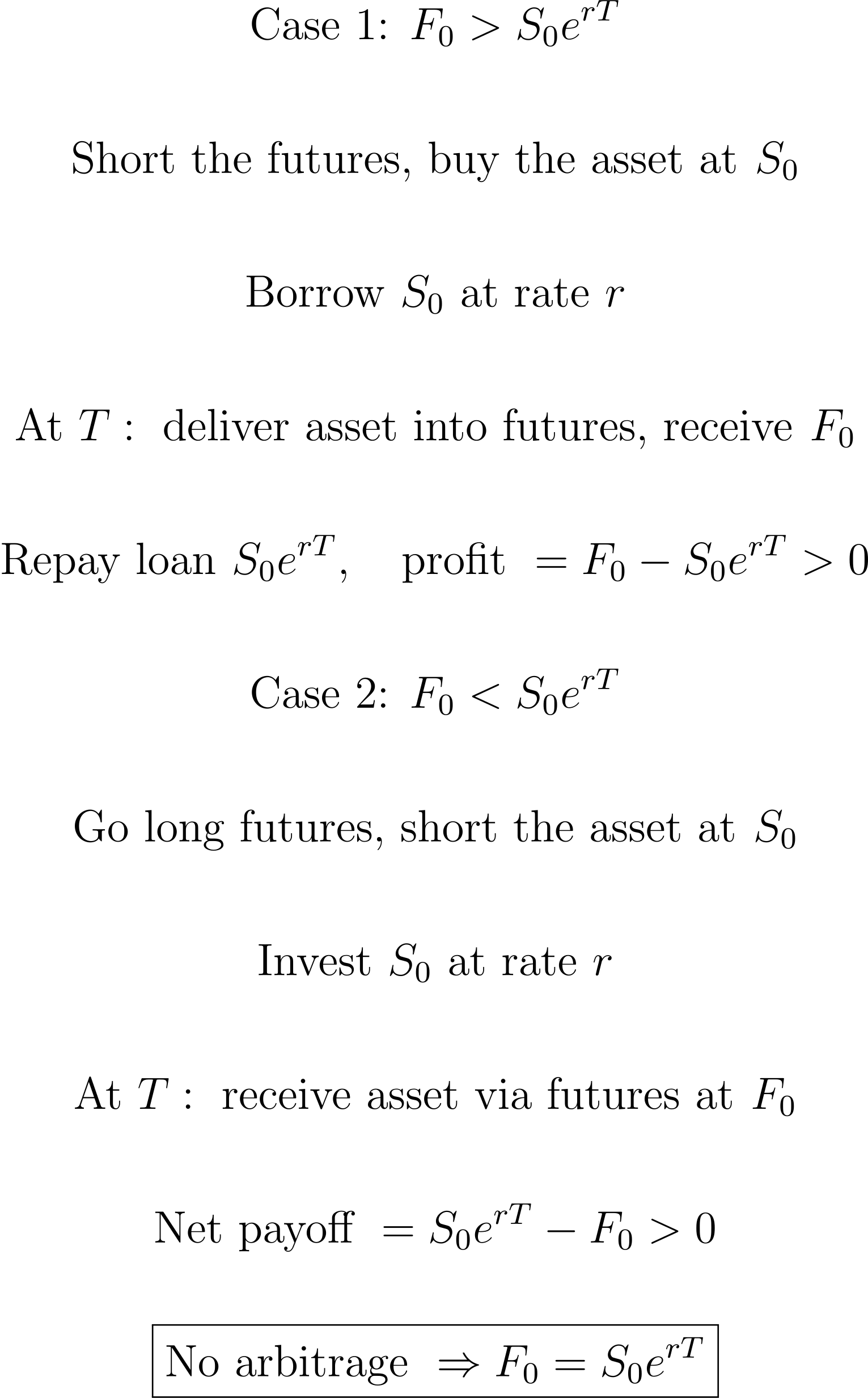
Events in markets tend to cluster, feeding on their own aftermath. The idea that arrivals are isolated and independent breaks down the moment activity picks up. That’s where the Hawkes process comes in. If the Poisson process is the clean baseline for random arrivals, the Hawkes process is what happens when you let arrivals influence future arrivals. Each event temporarily increases the likelihood of more events showing up soon after. Activity begets activity. Calm begets calm. It’s a small but powerful shift that turns a memoryless arrival model into one with feedback. You can think of Hawkes processes as Poisson processes with memory. The arrival rate isn’t fixed, it responds to the past. This makes them a natural fit for modeling trade arrivals, order flow, quote updates, price jumps, volatility bursts, and anything else in markets where one event tends to trigger more. If you’ve seen my previous video on Poisson arrival processes, this is the next step: same foundation, richer dynamics. I’ll be covering Hawkes processes more formally on the YouTube channel down the line, but for now, the key idea is simple: markets don’t just have events, they amplify them. Here’s what the Hawkes structure looks like: |
A Hawkes process takes that idea one step further and applies it to events themselves. Instead of modeling how values respond to past shocks, a Hawkes model says that each event changes the likelihood of future events arriving. A trade doesn’t just print and disappear into history, it temporarily raises the intensity of more trades. A volatility spike doesn’t just happen, it makes additional spikes more likely in the near future. The baseline intensity represents the background rate of activity, while the excitation kernel controls how strongly and how long each event feeds back into the system. Unlike a simple Poisson process, arrivals are no longer independent; activity creates more activity, until the influence decays and the system relaxes. Depending on the shape and strength of that excitation, events can cluster tightly, cascade, or fade quickly back to baseline. In one line, the Hawkes process captures a different truth about markets: events don’t arrive in isolation, they trigger aftershocks. This is why Hawkes models show up naturally in order flow, trade arrivals, jump timing, and volatility bursts, anywhere the market seems to “wake itself up.” And yes, this dynamic is sitting quietly underneath a lot of trading intuition people apply without realizing it. When traders talk about “momentum in flow,” “activity picking up,” or “the tape heating up,” they’re implicitly describing self-excitation. Like technical indicators, Hawkes models can work, stop working, then start working again, the hard part isn’t using them, it’s understanding why the feedback loop is present, when it breaks, and how long it lasts. That’s where modeling stops being about signals and starts being about structure. |
📈 Model applications Hawkes processes are used when the timing of events matters just as much as their occurrence. They’re especially effective in markets where activity clusters: trades triggering more trades, volatility spikes followed by more volatility, order flow accelerating once it starts moving. A Hawkes model says “an event increases the chance of more events,” which immediately explains why markets feel quiet for long stretches and then suddenly explode with activity. This makes them a natural fit for modeling trade arrivals, order submissions, cancellations, quote updates, and jump timing in prices. What Hawkes models do particularly well is separate baseline activity from feedback. There’s a steady background rate of events, but each arrival temporarily excites the system, raising the intensity before it decays back down. That structure captures how markets digest information in bursts rather than smoothly. News doesn’t arrive and disappear; it propagates through flow, liquidity, and reactions. When excitation is strong, you see cascades. When it’s weak, the market quickly calms down. The model makes those dynamics explicit. Like MA models, the real value of Hawkes processes isn’t that they’re “correct,” but that their assumptions are visible. They assume clustering comes from self-excitation rather than pure randomness. When activity suddenly stops clustering, or when excitation parameters shift, the model breaks, and that break itself is informative. In practice, Hawkes processes aren’t endpoints; they’re components. They’re embedded inside execution models, microstructure simulations, jump-diffusion timing, and systemic risk analysis. They work as long as the market feeds on its own activity, and when that changes, the model tells you the regime has changed with it. 🎓 A little story When I first started studying time-inhomogeneous Poisson processes in any real depth, it genuinely stopped me in my tracks. Everything I had instinctively disliked about early models (strict stationarity, constant parameters, pretending the world behaves the same on Monday as it does during a crisis) was finally being addressed head-on. The arrival rate itself was allowed to move. Intensity could breathe with time. The model acknowledged, explicitly, that markets speed up, slow down, and change character depending on what’s happening around them. That was a big moment for me. Up until then, so much of time-series modeling had felt like a careful dance around assumptions everyone knew were wrong but tolerated anyway. Time-inhomogeneous processes flipped that on its head: instead of forcing reality into a static box, the box moved. Activity could surge during news, fade in calm periods, and evolve structurally without pretending the system was stationary underneath. Hawkes processes felt like the natural next step. Not only does the intensity vary through time, but events themselves shape that variation. Activity feeds on activity. Calm reinforces calm. It’s the same idea pushed one layer deeper, a model that doesn’t just accept time variation, but explains why it emerges. Seeing that progression made something clear to me: good models don’t deny instability, they organize it. They don’t freeze the world in place; they give you a framework for understanding how it changes. That realization tied together a lot of threads from years of study. Models aren’t about finding something that “always works.” They’re about building structures that adapt, fail loudly when regimes shift, and help you prepare rather than predict. Time-varying intensity wasn’t just a technical improvement, it was an acknowledgment of how markets actually behave. 💡 Takeaway Every model we write is wrong in some way. The only real question is how it’s wrong and whether it’s wrong in a useful direction. Model specification isn’t about finding truth; it’s about choosing assumptions that capture the dynamics that matter for decision making. We’re always approximating a world that’s more complex, more adaptive, and more unstable than any equation can fully describe. Hawkes processes are a good example of getting that tradeoff right. They don’t pretend arrivals are independent or uniformly random. They acknowledge something we see constantly in markets: events cluster. Trades trigger trades. Volatility begets volatility. Activity feeds on itself. By parameterizing that feedback explicitly, Hawkes models move us closer to how markets actually behave, without pretending we’ve solved the system. So no, Hawkes processes aren’t “correct” in some absolute sense. But they’re correct in structure. They encode the idea that risk often comes from bursts, cascades, and aftershocks rather than isolated events. And when you improve that structure, allow intensities to evolve, excitation to decay differently across regimes, or parameters to shift through time, everything downstream improves with it: execution models, risk estimates, stress scenarios, and intuition. Good models don’t eliminate uncertainty. They organize it. And Hawkes processes do exactly that by admitting a simple, powerful truth: markets remember their own activity, and clustering isn’t noise, it’s structure. |
🏆 Quant Question of the Week |
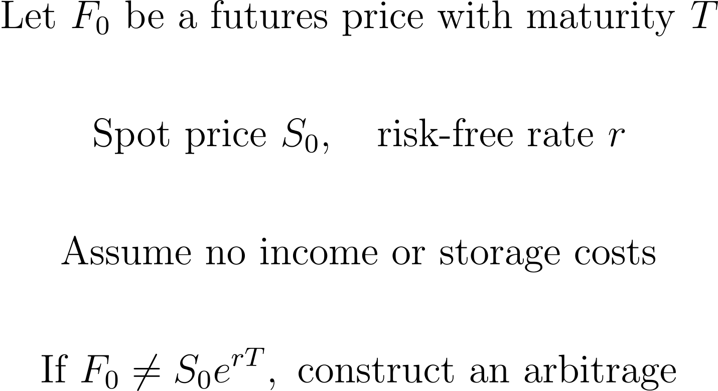
Solution at the Bottom of this Email 👇 |
Need to study up on topics in math, probability, and finance? 👉 Learn to solve problems like this on Quant Guild — the platform I wish I had when I was studying to become a quant. |
📅 Quant Guild Week in Review |
Risk-Neutral Pricing and Live Volatility Surfaces |
|
|---|
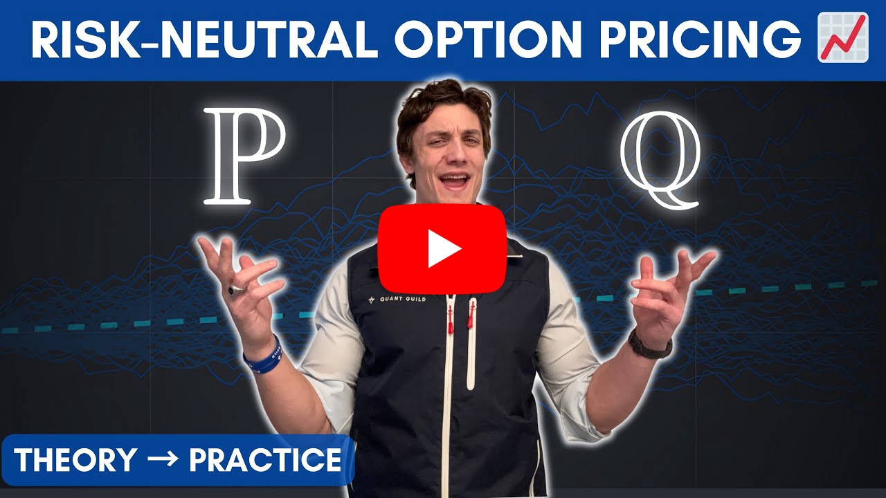
📈 Quant Explains Risk-Neutral Option Pricing | In this video I explain how options can have a single fair price even when two market participants have completely different beliefs about where the underlying asset is going. I start with a simple market-making problem. You think the stock is going to the moon, I don’t. So how do we agree on a price? The answer is that pricing derivatives is not about speculation. It is about no-arbitrage consistency, and that leads directly to the idea of risk-neutral pricing. I begin by walking through European option payoffs and showing why pricing is inherently probabilistic. The payoff is known at maturity, but the terminal stock price is not. To deal with that uncertainty, we introduce stochastic models like geometric Brownian motion and simulate possible future price paths. This immediately raises two major real-world issues: model misspecification and model misparameterization. Different assumptions or estimation windows can produce wildly different distributions and wildly different prices, which makes naïve pricing frameworks unstable. This is where risk-neutral pricing enters. I explain the change of measure from the real-world probability measure P to the risk-neutral measure Q. A change of measure is simply a change in distribution. Under the risk-neutral measure, the expected return of the underlying is the risk-free rate, not because we believe it will earn that rate, but because the Black-Scholes replication argument constructs a portfolio that removes hedgeable risk entirely. With randomness cancelled out, the remaining portfolio must earn the risk-free rate by no-arbitrage. I connect this directly to the Black-Scholes PDE, the Fundamental Theorem of Asset Pricing, and the Feynman–Kac theorem, showing why Monte Carlo simulation with risk-free drift converges to the Black-Scholes price. I also address a major source of confusion: why we simulate with the risk-free rate rather than zero drift, even though the replicating portfolio itself is risk-free. The key is that the simulated process represents the risk-neutral dynamics of the underlying, not the hedged portfolio. From there, I move beyond the classroom case. Real markets are incomplete. There are jumps, stochastic volatility, and unhedgeable risks. That means there are infinitely many risk-neutral measures. Instead of choosing one arbitrarily, we infer the appropriate risk-neutral measure by calibrating models to market prices of liquid options. This calibration process produces the implied volatility surface and explains why skew exists. Downside risk cannot be hedged away, so it commands a premium. The core takeaway is that risk-neutral pricing is not about believing the market is rational or models are correct. It is about building a consistent pricing framework in the presence of uncertainty, misspecification, and unhedgeable risk. Even in the risk-neutral world, modeling risk never disappears. It simply changes form. Understanding that distinction is what separates surface-level option pricing from real quantitative finance. | | | 🎲 Building Live Volatility Surfaces in Python | In this video I explain why volatility surfaces sit at the center of modern options trading and stochastic modeling, and why most retail traders never interact with them properly. Large institutions have effortless access to clean, real-time volatility surfaces. They use them constantly for model calibration, pricing exotics, managing risk, and identifying mispricings. Retail traders, on the other hand, are usually stuck looking at single implied volatility numbers or static charts with no connection to theory or execution. I start by explaining what a volatility surface actually represents. It is not just a visualization. It is the market’s collective pricing of uncertainty across strike and maturity. Every stochastic volatility model, every jump diffusion, every local volatility framework is ultimately trying to explain and reproduce this object. If you want to do serious options trading or model calibration, you cannot treat the surface as something abstract or external. You need to construct it yourself, understand how it evolves, and observe it live. The core idea of the video is that retail traders are not blocked by theory. They are blocked by infrastructure. Institutions infer the risk-neutral measure directly from the volatility surface and recalibrate constantly. As retail participants, if we want to operate in the same conceptual framework, we need to build the surface ourselves in real time using live option quotes. That is what bridges the gap between textbook financial mathematics and real trading systems. This video demonstrates that bridge. It shows how to go from raw option prices to a live volatility surface that can be used for stochastic calibration, regime analysis, and trading decisions. To my knowledge, this is the only video online that explicitly connects the theory of risk-neutral pricing and volatility modeling to a working real-time retail system. The goal is not just to visualize volatility, but to give retail traders access to the same objects institutions rely on every day. | | |
|
|
|---|
|
 | 📈 Why 10,000+ Quants Study on Quant Guild | Quant Guild is the one-stop platform for mastering the math that powers modern finance. With 90+ specialized lessons, adaptive practice with gamified progress that scales with your skill level, real interview questions, courses from A - Z in coding, math, probability & statistics, and exclusive live classes with me, it’s built to take you from fundamentals to the front-office. Everything’s designed for how real quants think and work — focused, practical, and deeply technical. That’s why over 10,000+ students and professionals study on Quant Guild to sharpen their edge and make smarter decisions in the face of uncertainty. | 🏛️ See How Pol Became a Market-Maker with Quant Guild | 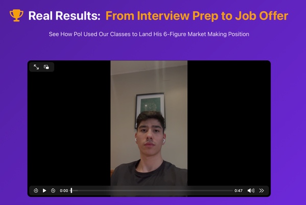 |  |
|
|
|---|
| | I'm in QR preparing for technical interviews and your practice helped me brush up on probability, thanks | | |
| | |
|
| | | I learned more here in two days than an entire semester of college | | |
| - Guy on Discord Who DM'd Me |
|
|
|
|---|
|
| | ✅ Quant Question of the Week |
| | | | | | |
|
|
|---|
|

 Roman Paolucci