 | | | 📜 A Note from the Guild Leader |
| There are a few seats left for the next live class session on Quant Guild: Computational Finance. This class meets twice a week and prioritizes the quantitative toolkit necessary for advanced coursework in post-graduate academic programs and industrial roles in trading and market-making. | | | Interested in learning more? Check out the syllabus below! | - Week 1: Mathematics
- Calculus: Derivatives, Partial Derivatives, Gradient Vectors
- Numerical Computing of Integrals and Gradients
- Linear Algebra: Matrices, Vectors, Spaces, Subspaces, Span
- Linear Independence, Determinants, Matrix/Scalar Multiplication
✔ Homework + Numerical Linear Algebra Project - Week 2: Probability and Statistics
- Random Variables, Max Likelihood Estimation (MLE)
- Law of Large Numbers (LLN) & Central Limit Theorem (CLT)
- Stochastic Processes: Markov Chains & Poisson Processes
- Introduction to Brownian Motion
✔ Homework + Stochastic Modeling Project - Week 3: Machine Learning
- Linear Regression & How Machines Learn
- The Machine Learning Pipeline
- Parameter/Model Misspecification & Non-stationarity
✔ Homework + Regression Analysis Project - Week 4: Applications of Quantitative Topics I
- Pricing Financial Derivatives (Options Pricing Models)
- Modeling Exogenous Events
- Constructing and analyzing a Portfolio of Bonds
✔ Homework + Options Pricing Engine - Week 5: Applications of Quantitative Topics II
- Portfolio Management: CAPM, Fama-French, Factor Modeling
- Quantitative Trading: Research Pipeline Overview
- Applications of AI/ML in the industry
✔ Homework + Factor Modeling Project
| | | Students have permanent access to session recordings, course materials/projects and their accompanying solutions. Interested in enrolling? Check out Computational Finance on the Live Classes page on Quant Guild! | With that I will leave you to the Weekly Guild Letter. I hope you enjoy, and I hope you learn something! - Roman | | | 🧮 Quant Model of the Week |
| Goldman Sachs, Variance Swaps, and the VIX |
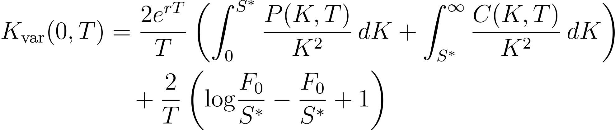
| Variance swaps are one of those instruments that look simple on the surface and become profound the moment you unpack them. At first glance, it is just a contract on realized variance. No direction. No delta. Just a pure trade on how much the underlying actually moves. But the pricing formula, especially the one popularized in the Goldman Sachs desk note on Emmanuel Derman’s website, reveals something deeper. Variance is not priced by forecasting volatility directly. It is replicated. The key insight is that a variance swap can be statically replicated using a strip of out-of-the-money options across strikes. Instead of predicting realized variance, you extract its fair value from the implied volatility surface itself. The model-free replication result connects realized variance to a weighted integral of option prices. It is one of the cleanest demonstrations of how no-arbitrage and replication arguments turn uncertainty into something tradable. This formula sits at the intersection of theory and practice. It links the abstract idea of quadratic variation to actual listed options on a screen. It shows how desks price volatility not by guessing, but by constructing. And once you see it, you start recognizing the same principle everywhere in derivatives: if you can replicate it, you can price it. Let’s walk through the formula and see what is really going on. | | | At a high level, the variance swap pricing formula comes from a replication argument. Under a standard diffusion, the realized variance is tied directly to the quadratic variation of log returns. If you apply Itô’s lemma to the log of the price process, you discover that realized variance can be expressed through a combination of a continuously rebalanced stock position and a static position in a log contract. The stock component is straightforward. Under diffusion assumptions, we can dynamically hedge that part by continuously rebalancing the underlying. That piece is mechanical. The harder part is the log payoff. We cannot directly trade a log contract. This is where the Carr–Madan spanning result enters. It tells us that sufficiently smooth payoffs, including the log payoff, can be statically replicated using a strip of options across strikes. That is exactly what the two integrals over puts and calls are doing. We use out-of-the-money options only, both for liquidity and to avoid redundancy, since in-the-money options can be decomposed into out-of-the-money options plus forwards. The hinge point S∗ splits the integration between puts and calls. In practice, it is often chosen at or near the forward. The adjustment term involving the log and forward ensures the replication matches the annualized realized variance exactly. It corrects for the fact that we are replicating the log payoff around a finite hinge point rather than integrating over an idealized continuum. The final expression gives the fair delivery price of variance, annualized and risk-neutral. It is not a forecast. It is a no-arbitrage construction extracted from the option surface itself. That is the elegance of the formula: realized variance becomes tradable because it can be replicated. | 📈 Model applications The most famous application of this formula is the VIX. At its core, the VIX is nothing more than the fair strike of a 30-day variance swap on the S&P 500, expressed in volatility terms. The CBOE implementation uses exactly this replication logic. Instead of forecasting future volatility, it extracts the market’s risk-neutral expectation of future variance from a strip of out-of-the-money options across strikes. | | | The integrals in the formula become a discrete sum over listed SPX options. Deep out-of-the-money puts capture downside tail risk. Out-of-the-money calls capture upside participation. Together, weighted appropriately by 1/K^2, they replicate the log payoff and therefore the expected quadratic variation. The result is an annualized variance measure. Take the square root, scale appropriately, and you have the VIX index. What makes this powerful is that it is model-free under diffusion assumptions. No GARCH. No Heston calibration. No subjective volatility forecast. The market tells you its implied variance directly through option prices. In that sense, the VIX is not a prediction in the traditional sense. It is a tradable consensus, backed out from the option surface via replication. This is why variance swaps and the VIX sit at the center of volatility trading. They provide a clean bridge between theory and the screen. The formula tells you the fair delivery price of variance. The option market tells you where it is actually trading. And the gap between the two is where trading, hedging, and relative value strategies live. 🎓 A little story The first time I saw replication was in a one-period binomial tree. Two possible states. Pick the right combination of stock and bond. Match the payoff exactly. If you can replicate the derivative in every state of the world, then it must cost the same as the replicating portfolio. Otherwise, free money. End of story. At the time, it seemed like a neat classroom trick. Elegant, yes. Powerful, maybe. But still small. Then I saw the same idea again in continuous time through the Black–Scholes argument. Delta hedging. Continuous rebalancing. Eliminate risk locally. Force the portfolio to earn the risk-free rate. The binomial logic had not disappeared. It had just been refined. The tree became a diffusion. The hedge became dynamic. The intuition stayed the same. If you can replicate it, you can price it. And if you can price it under a risk-neutral framework, you can make a market in it. Suddenly it was not just calls and puts. It was variance. Correlation. Skew. Volatility-of-volatility. Tail risk. Anything that could be expressed as a payoff and functionally replicated had a theoretical fair value. The realization was bigger than the math. Pricing was not prediction. It was construction. And once you understand that, you start seeing derivatives not as exotic bets, but as engineered exposures. If you can define the payoff and build the hedge, you can quote a price. That is not just theory. That is how desks operate every day. 💡 Takeaway A lot of the numbers that dominate financial headlines are not mystical gauges of fear. They are artifacts of replication. The VIX is a perfect example. It is not a crystal ball. It is not a survey of sentiment. It is the fair strike of a variance swap, extracted mechanically from option prices using a no-arbitrage argument. It exists because we can replicate a log payoff with a strip of options and continuously hedge the underlying. That theoretical foundation is what gives it meaning. But in practice, many traders and commentators treat these constructs as standalone signals, detached from the structure that created them. They react to the level without thinking about the assumptions underneath, the liquidity conditions embedded in the option surface, or the risk-neutral framework that defines it. The broader lesson is this: markets generate measurable quantities that look fundamental, but they are often engineered outputs of pricing theory. If you do not understand the replication argument behind them, you are trading a headline. If you do understand it, you are trading structure. | | | 🏆 Quant Question of the Week |
| Solution at the Bottom of this Email 👇 |
| | | Need to study up on topics in math, probability, and finance? 👉 Learn to solve problems like this on Quant Guild — the platform I wish I had when I was studying to become a quant. | | | 📅 Quant Guild Week in Review |
| Pricing Variance Swaps and Kalman Filters |
|
|
|
|---|
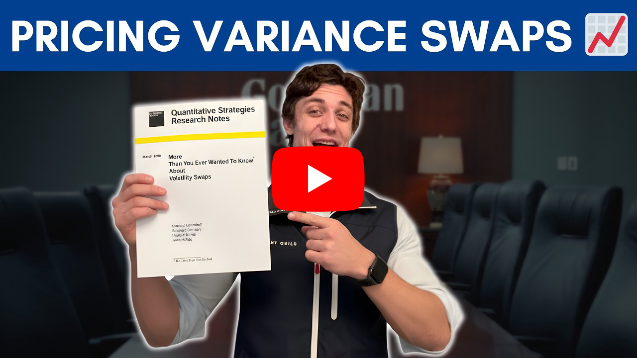
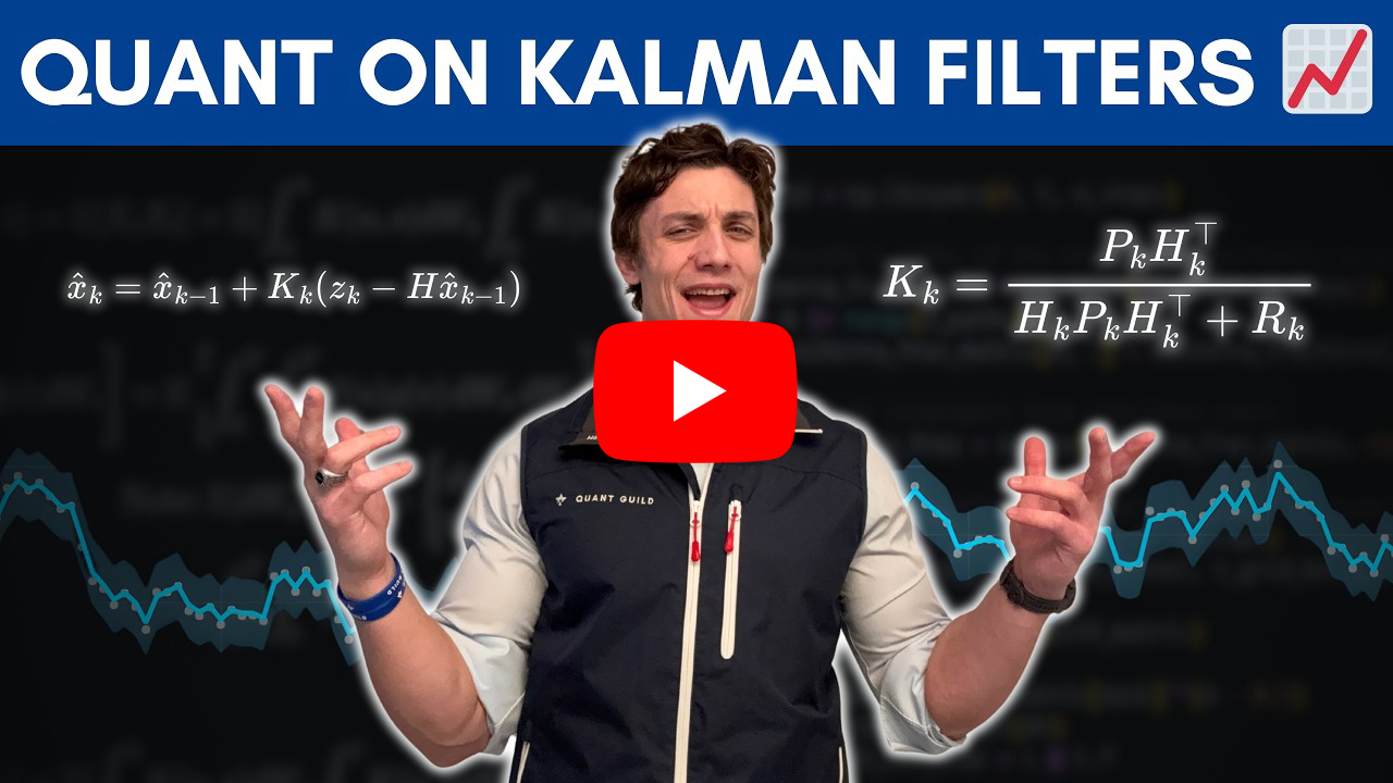
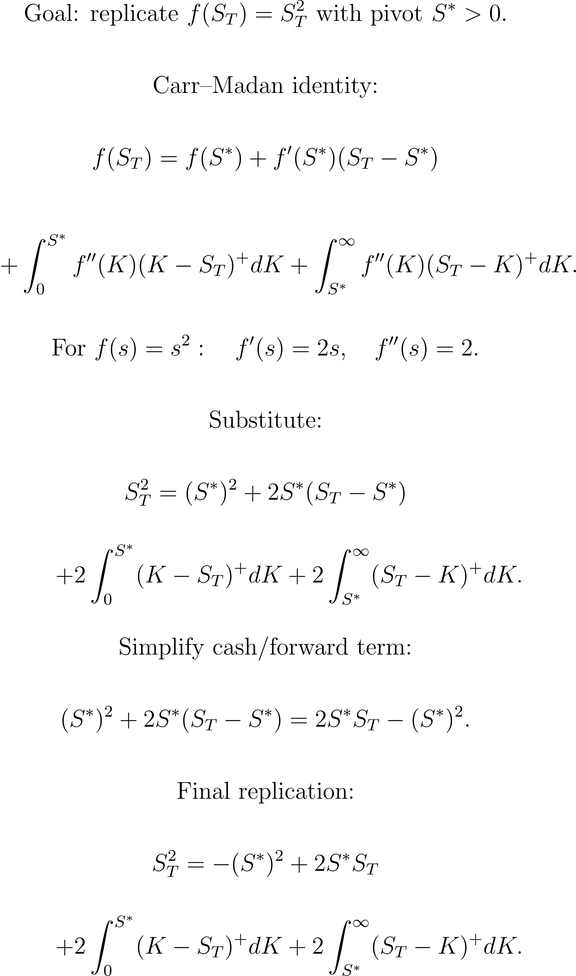
📈 How Goldman Sachs Prices Variance Swaps | In this video I walk through how Goldman Sachs derived the risk-neutral pricing formula for variance swaps and why it’s one of the most elegant arguments in quantitative finance. I start by explaining what a variance swap actually is. It’s just a forward contract on annualized realized variance. If you’re long, you profit when realized variance exceeds the implied variance strike. If you’re short, you profit when realized variance comes in lower. There’s no physical delivery. It’s simply a cash settlement at maturity based on the difference. From there, I derive the fair delivery price using arbitrage pricing theory. I assume standard diffusion dynamics for the underlying and define realized variance as the time integral of squared volatility. Then I apply Itô’s lemma to a log transformation of the price process. This is the key step. It allows me to express realized variance in terms of tradable objects: a continuously rebalanced position in the underlying and a short position in a log payoff. That transformation is what connects stochastic calculus to something you can actually trade. Next, I move to the risk-neutral measure. Under no-arbitrage, the continuously rebalanced stock component earns the risk-free rate in expectation. What remains is the short log payoff. But we can’t trade a log payoff directly. This is where the Carr–Madan replication theorem comes in. Any twice-differentiable payoff can be replicated with an infinite strip of out-of-the-money calls and puts. By expanding the log payoff around a hinge point, we decompose it into weighted integrals of calls and puts across strikes. When we combine everything, we obtain the implied variance strike as a function of observable option prices. In other words, variance is not priced by guessing volatility. It is priced by constructing a synthetic portfolio of options that replicates the log contract. This is the same structural logic behind the VIX and the Goldman Sachs desk notes from the 1990s. The core takeaway is that variance swaps are not mystical volatility products. They are a direct consequence of no-arbitrage, stochastic calculus, and option replication. Once you see the derivation, you realize the entire object is just a carefully engineered portfolio of tradable instruments. Here's a link to the full video 👇 | | | 🎲 Kalman Filters for Quant Finance | In this video I explain why every quant faces a model specification and parameterization problem, and how the Kalman filter helps us manage that reality in live systems. Anytime we build a model, whether it’s linear regression, AR processes, GARCH, or mean reversion, we are making assumptions about structure and parameters. Even if the model is rooted in solid economic theory, it can still fail due to misparameterization or regime change. And when it fails, every probability, forecast, and expected value built on top of it becomes unreliable. I motivate this using volatility modeling, specifically the VIX. Volatility is well documented to be mean reverting. If you ignore that and fit a naïve linear model, your forecasts explode to unrealistic extremes. But even if you choose the correct structure, like an Ornstein–Uhlenbeck process, poor parameterization can make rare but very real events look impossible. That’s the danger. Specification and parameterization sit upstream of every decision we make under uncertainty. The Kalman filter enters as a dynamic reconciliation mechanism. It combines a model rooted in theory with noisy real-world observations to estimate the true underlying state. Instead of blindly trusting the model or blindly reacting to every new print, the filter balances both using the Kalman gain. If measurement noise is low, we lean into the data. If model uncertainty is low, we lean into theory. This trade-off becomes critical during regime shifts, where being too reactive causes whiplash and being too rigid causes stale forecasts. I walk through the full state space framework, showing how we calibrate an offline model first, initialize uncertainty, and then recursively update forecasts as new data arrives. The key insight is that the standard Kalman filter updates the state, not the underlying model parameters. If the regime truly changes, you may need dual-filter or extended approaches that update both the state and the parameterization itself. Otherwise, you are applying a band-aid to a broken structural assumption. I close by connecting this to real institutional use cases, including volatility modeling and illiquid bond pricing. The Kalman filter shines whenever you have a theoretically grounded pricing model but incomplete or noisy observations. It provides a disciplined way to combine structure and data in real time. The overarching takeaway is simple. Models will break. Parameters will drift. The question is whether your system adapts intelligently or continues producing misleading probabilities. The Kalman filter is one of the most powerful tools we have for bridging theory and live market reality. Here's a link to the full video 👇 | | |
|
|
|---|
|
 | 📈 Why 10,000+ Quants Study on Quant Guild | Quant Guild is the one-stop platform for mastering the math that powers modern finance. With 90+ specialized lessons, adaptive practice with gamified progress that scales with your skill level, real interview questions, courses from A - Z in coding, math, probability & statistics, and exclusive live classes with me, it’s built to take you from fundamentals to the front-office. Everything’s designed for how real quants think and work — focused, practical, and deeply technical. That’s why over 10,000+ students and professionals study on Quant Guild to sharpen their edge and make smarter decisions in the face of uncertainty. | 🏛️ See How Pol Became a Market-Maker with Quant Guild |  |  |
|
|
|---|
| | I'm in QR preparing for technical interviews and your practice helped me brush up on probability, thanks | | |
| | |
|
| | | I learned more here in two days than an entire semester of college | | |
| - Guy on Discord Who DM'd Me |
|
|
|
|---|
|
| | ✅ Quant Question of the Week |
| | | | | | |
|
|
|---|
|

 Roman Paolucci