 | | | 📜 A Note from the Guild Leader |
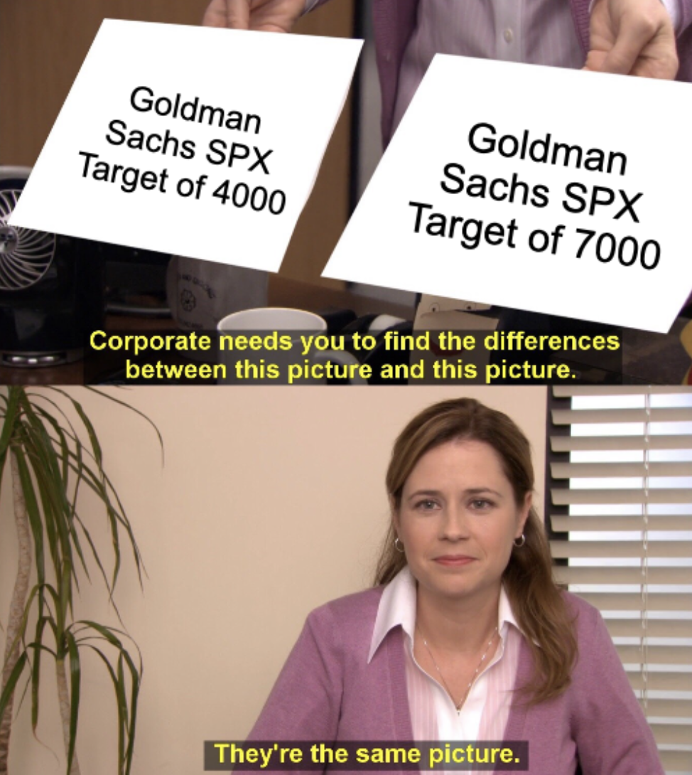
| Models are always wrong, that's not a hot take. I am, however, more critical than most of all forward looking probabilities, statistics, and similar measures. That's because I've seen it far too many times: - "My indicator said to buy" - "The price target was $300" - "Banks were all long SPX this year" all this "information" and misinformed traders are stuck with the bill when they never actually understood the price of the menu items they ordered. | | | The necessary mathematical background to understand these models and measures is vast. It takes a very many number of years to be capable of comprehending assumptions, violations, and implications of violated assumptions in practice. Anyone who suggests otherwise is either naive, egotistical, or trying to sell you something. Which is why I hate these measures. They're an arbitrary compression of best guesses. We can all pull up the analyst price targets for equities and ETFs, but do you know what they mean? Literally nothing. Some use these to inform their decision making, maybe they offer some cross-sectional explainability in variation, but that's still an artifact of data and ephemeral at best. As crisis unfolds in realtime you will find these targets are immediately lowered...yeah, no kidding. When you understand the markets through the lens of non-stationarity you begin to ask the right questions about out-of-sample stability, performance under varying regimes, so on and so forth. If these questions bore you then you are effectively (and likely) triple long; placing your job, house, and 401K on red (macro) which is always subject to change. This is why we all have jobs, managing capital is a full time job if you want to do it effectively. That'll do it for my quant rant this week on forward measures. | With that I will leave you to the Weekly Guild Letter. I hope you enjoy, and I hope you learn something! - Roman | | | 🧮 Quant Model of the Week |
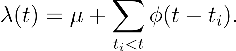
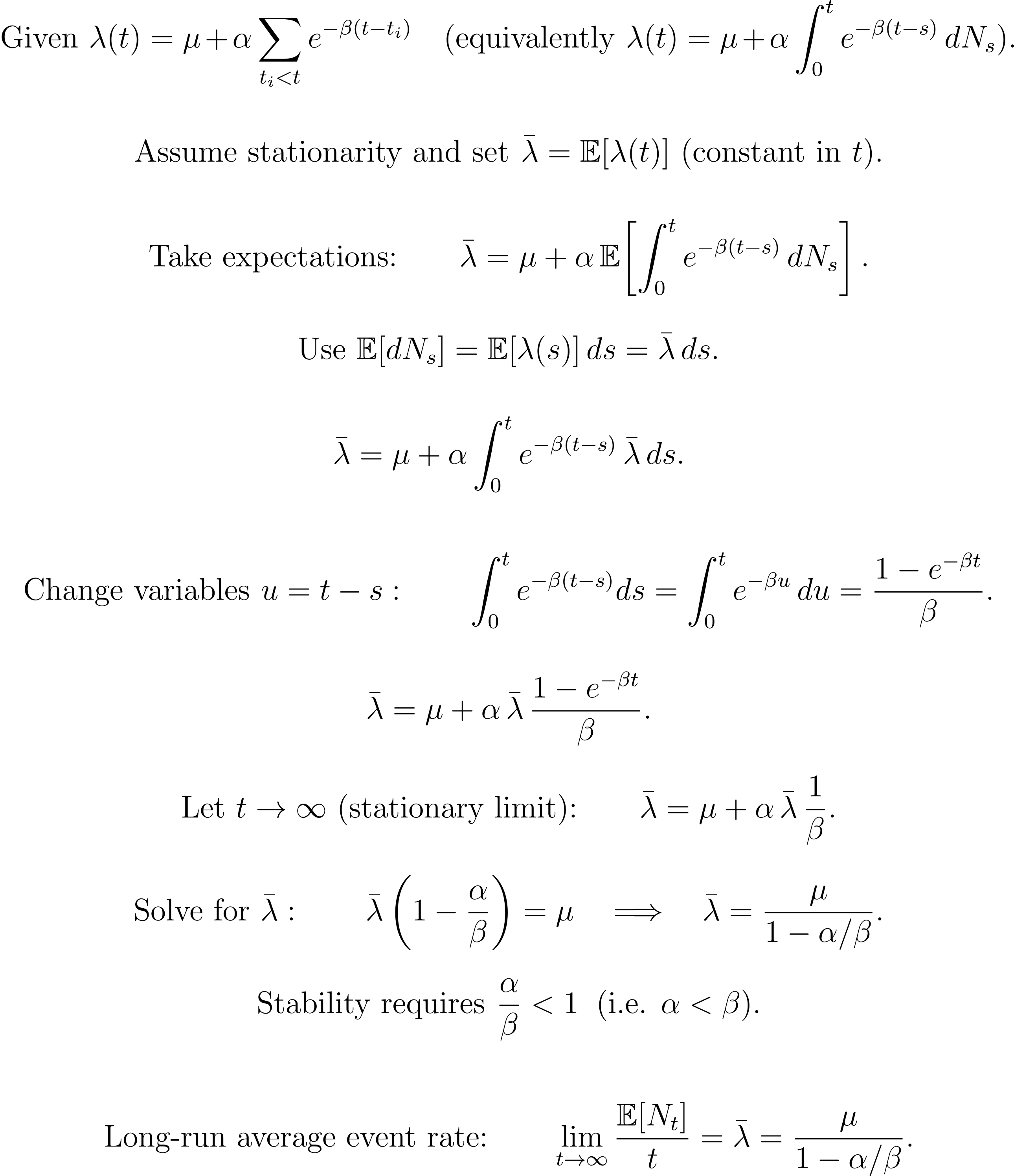
| | | Markets clearly exhibit excess kurtosis. Jump diffusion models capture fat tails well by adding Poisson-driven jumps to a diffusion. But standard jump processes assume independence. One jump does not influence the next. That misses something critical. In real markets, activity clusters. Selloffs trigger more selling. Volatility spikes beget more volatility. The arrival of one event increases the likelihood of more events in the near future. Hawkes processes model exactly this self-exciting behavior by letting the jump intensity depend on past jumps. They are used to model trade arrivals, order flow, price jumps, volatility bursts, and contagion effects in risk systems. Anywhere activity feeds on itself, Hawkes processes provide a more realistic structure than independent Poisson arrivals. This is what the stochastic intensity function looks like. | | | At the heart of the Hawkes process is the stochastic intensity function. It is no longer constant. It moves. There are two core components. First, a baseline rate, usually denoted by μ. This is the background intensity. If nothing happens, arrivals still occur at this steady, exogenous rate. Think of it as normal market activity when nothing unusual is going on. Second, a triggering kernel, often written as φ. This term captures self-excitation. Every time an event occurs, it temporarily increases the intensity. The shape and decay of φ determine how strongly and how long past events influence future arrivals. If the kernel decays quickly, clustering is brief. If it decays slowly, activity persists. Baseline activity plus feedback. That combination is what turns a memoryless Poisson process into a self-exciting one. | 📈 Model applications In practice, Hawkes processes are used anywhere timing and clustering matter. Banks use them to model trade arrivals, order book activity, and execution risk. If flow is self-exciting, then liquidity conditions can deteriorate quickly. Modeling clustering helps desks price impact, manage inventory, and avoid getting run over when activity accelerates. On the risk side, funds use Hawkes-style dynamics to model jump clustering and volatility bursts. A single shock rarely comes alone. Modeling self-excitation improves tail risk estimates, stress testing, and scenario generation because it captures contagion rather than isolated events. In short, Hawkes processes help institutions quantify feedback loops. When markets wake up and start feeding on their own activity, this framework makes that amplification explicit instead of pretending shocks arrive independently. | 🎓 A little story The first time I learned about stylized facts like volatility clustering and the leverage effect, my modeling world expanded overnight. Prices were not just diffusions. Volatility was not constant. Shocks were not isolated. Returns had memory in their second moments. Down moves lifted volatility. Activity fed on itself. I immediately wanted to build models that captured all of it. Every feature. Every empirical artifact. No compromises. Then I ran into reality. When I first saw PCA, and the idea of explained variance, something clicked. You rarely need one hundred percent of the variation. In fact, chasing it usually means you are fitting noise. A handful of components can explain most of what matters. Enough structure to accomplish the task at hand. Enough fidelity to make better decisions. Not perfection. That realization reshaped how I thought about modeling. The goal is not to capture every dynamic. It is to capture the dynamics that matter for pricing, hedging, or risk. The rest is complexity for its own sake. Models are tools, not encyclopedias of reality. 💡 Takeaway We do not add self excitation to a model because it is mathematically cool. We add it because clustering materially changes risk. Volatility bursts are not random decorations on top of a diffusion. They alter tail probabilities, drawdown speed, liquidity risk, and execution cost. If your model assumes independent jumps when markets clearly amplify their own activity, you are underestimating danger. But at the same time, Hawkes is not “the final model.” It is one more dominant component. Just like PCA teaches us that a few principal directions explain most variation, Hawkes teaches us that clustering is one of the main structural drivers of extreme behavior. We do not need to capture every micro-dynamic of the market. We need to capture the ones that change decisions. The goal is not 100% realism. It is sufficient realism. Hawkes processes acknowledge that events trigger events. That single adjustment can dramatically improve tail modeling and risk assessment. That is the balance: not modeling everything, but modeling what actually moves the needle. | | | 🏆 Quant Question of the Week |
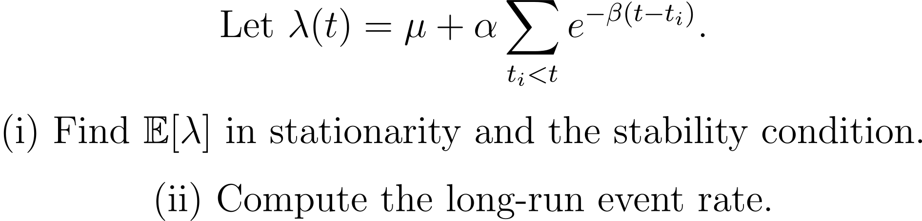
| Solution at the Bottom of this Email 👇 |
| | | Need to study up on topics in math, probability, and finance? 👉 Learn to solve problems like this on Quant Guild — the platform I wish I had when I was studying to become a quant. | | | 📅 Quant Guild Week in Review |
| Non-Stationarity, Why Market Timing Fails, Hawkes Processes |
|
|
|
|---|
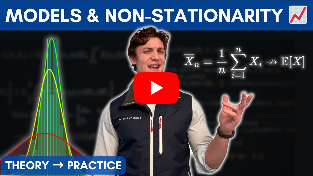
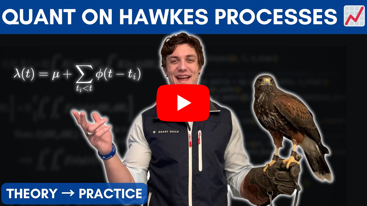
📈 Non-Stationarity and Why Market Timing Fails | The problem is that markets do not behave like a fixed dice. They are non-stationary. Regimes shift. Volatility changes. Structural breaks occur. The academic assumption of stationarity is a simplifying tool, not a property of reality. You cannot take something non-stationary and force it to become stationary. Markets are not neat probability distributions. They are the compressed outcome of countless decisions interacting over time. I illustrate this with a regime-switching example. You may estimate a fair value under one distribution, only to have the distribution change without warning. If you fail to adapt, your model becomes stale and your edge disappears. The real difficulty is that you do not observe the regime directly. You only observe returns. You do not know when the environment shifts, how much historical data is still relevant, or which parameterization is appropriate today. That is why market timing is so difficult. I also show how compressing returns into a single histogram hides this time-varying structure. What appears to be fat tails is often a mixture of low, medium, and high volatility regimes layered together. If you ignore that dynamic structure, you underestimate risk and overestimate stability. The key takeaway is that the objective is not stationarity. It is stability. A robust strategy should survive regime shifts or adapt when they occur. Market timing fails because it assumes we can confidently identify regime transitions in real time. In practice, we are always estimating under uncertainty while the distribution itself continues to move. Here's a link to the full video 👇 | | | 🎲 Hawkes Processes for Quant Finance | In this video I explain how we improve our models when we realize they are not capturing the dynamics we observe in real markets. Every time we build a model, we generate probabilities and statistics that we know are imperfect. The real question is how imperfect they are, because that determines the quality of our decisions under uncertainty. The Hawkes process is a perfect example of returning to the classroom to build a better model once we realize the original one is missing something important. I start from the ground up with Poisson random variables and Poisson processes. A Poisson random variable models the number of rare events in a fixed interval. A Poisson process lets us observe the arrival of those events over time. If the intensity parameter is constant, we get independent arrivals. If we allow the intensity to vary with time, we move to a time inhomogeneous Poisson process, which better reflects reality such as different trading activity at market open versus midday. But even that is not enough. Financial markets exhibit volatility clustering. Large moves tend to trigger more large moves. Selling begets selling. Activity feeds on activity. A time varying Poisson process still treats intensity as exogenous. It does not allow past events to increase the likelihood of future events. That is where the Hawkes process comes in. The Hawkes process is self exciting. The intensity function depends on past arrivals. A jump increases the probability of another jump, and that influence decays over time back to a baseline rate. This captures contagion and clustering directly. It reflects how markets actually behave during crashes and high stress periods. I then connect this to jump diffusion models. A standard jump diffusion can introduce excess kurtosis and fat tails, but it does not capture clustering. Jumps occur independently. When we replace the Poisson component with a Hawkes process, we get a Hawkes jump diffusion. Now jumps cluster. Tail risk becomes more realistic. The implied wait time for extreme events drops dramatically compared to a naïve normal assumption. The core takeaway is that better modeling of event arrivals leads to more realistic probabilities and better risk assessment. If we ignore clustering and contagion, we underestimate tail risk. The Hawkes process brings us closer to the dynamics we actually observe in markets and therefore leads to more informed decisions under uncertainty. Here's a link to the full video 👇 | | |
|
|
|---|
|
 | 📈 Why 10,000+ Quants Study on Quant Guild | Quant Guild is the one-stop platform for mastering the math that powers modern finance. With 90+ specialized lessons, adaptive practice with gamified progress that scales with your skill level, real interview questions, courses from A - Z in coding, math, probability & statistics, and exclusive live classes with me, it’s built to take you from fundamentals to the front-office. Everything’s designed for how real quants think and work — focused, practical, and deeply technical. That’s why over 10,000+ students and professionals study on Quant Guild to sharpen their edge and make smarter decisions in the face of uncertainty. | 🏛️ See How Pol Became a Market-Maker with Quant Guild |  |  |
|
|
|---|
| | I'm in QR preparing for technical interviews and your practice helped me brush up on probability, thanks | | |
| | |
|
| | | I learned more here in two days than an entire semester of college | | |
| - Guy on Discord Who DM'd Me |
|
|
|
|---|
|
| | ✅ Quant Question of the Week |
| | | | | | |
|
|
|---|
|

 Roman Paolucci