 | | | 📜 A Note from the Guild Leader |
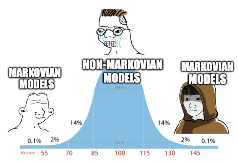
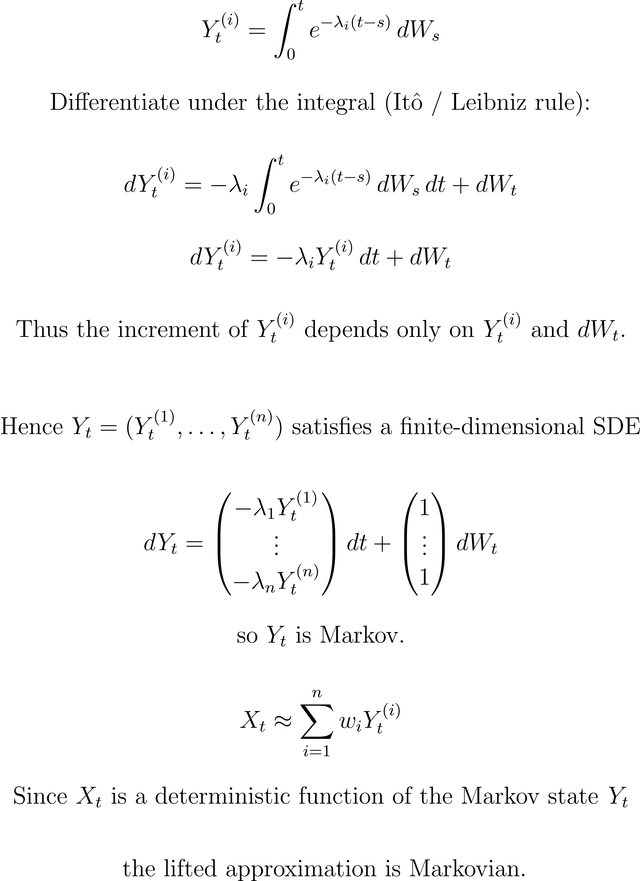
| If everything is path dependent why bother using a model that assumes the structure is Markovian? Non-Markovian models better capture empirical dynamics, though computationally intractable and useless on the desk we ought to use them, right? | | | Well Markovian structure isn't just a simplifying assumption but a desirable property of a model that may well still capture path dependence as I've discussed in my latest video: How Markovian Lifting Solves the Rough Volatility Problem. In other words, just because our non-Markovian models better capture empirical dynamics, it doesn't mean we can't implement approximations or other high fidelity compressions to recover this property (and subsequently affine structure). We are then back to our "simplifying assumption" but with path dependent dynamics enabling all the efficiency and tools of the assumption while still capturing the desired empirics. In any case, we all have to go through the middle of the curve to get back to the degen arbitrary model assumptions, but this time with extra steps making it actually (or at worst, more) valid. | With that I will leave you to the Weekly Guild Letter. I hope you enjoy, and I hope you learn something! - Roman | | | 🧮 Quant Model of the Week |
| | | Volatility does not behave the way classical models say it should. It is not smooth. It is not Markovian. It does not revert cleanly with a single time scale. When you look at high-frequency data, volatility is jagged, persistent, and rough, with shocks that decay slowly rather than exponentially. Gatheral’s 2014 work on rough volatility formalized this observation. Instead of modeling volatility as a smooth diffusion, it treats it as a process with fractional structure, capturing long memory and irregular paths. The result is a model that matches the empirical behavior of realized volatility far better than traditional stochastic volatility frameworks. | 🧮 Model Definition | This is what the rough volatility models empirical dynamics as... | | | What you’re looking at is a statement about how volatility increments scale over time. The expected squared change in volatility over a time step Δ grows like Δ raised to the power (2H). If H were 0.5, you would recover standard Brownian scaling. But empirically, H is much smaller, around 0.1. That means volatility paths are much rougher, with more short-term variability and stronger persistence than classical models assume. This behavior is modeled using a power law kernel. Instead of shocks decaying exponentially, as in standard mean-reverting models, their influence decays slowly according to a power law. Recent shocks matter a lot, but past shocks never fully disappear, they fade gradually over many time scales. That slow, scale-free decay is what generates the roughness. It embeds long memory directly into the volatility process and reproduces the empirical scaling observed in real data. | 📈 Model Applications | Rough volatility models are used where realistic volatility dynamics matter most. On derivatives desks, they improve the modeling of the volatility surface, especially short-term options, by capturing the steep skews and term structure that classical models struggle with. Because rough volatility matches the observed behavior of realized volatility, it leads to better pricing and hedging of options sensitive to short-dated moves. They are also critical for risk management and simulation. By incorporating long memory and persistent shocks, rough models generate more realistic volatility paths, improving scenario analysis, tail risk estimation, and stress testing. In short, rough volatility helps institutions align models with data. Instead of forcing volatility into smooth, Markovian dynamics, it captures the jagged, persistent behavior markets actually exhibit, leading to more accurate pricing and more honest risk assessment. | 🎓 A Little Story | At one point in an industrial research setting, I was completely focused on calibration. The problem felt obvious: these models are only as good as how fast and accurately you can fit them to market data. So naturally, I leaned into machine learning. Build an MCA-style approach, learn the mapping from parameters to prices, invert it efficiently, and you have near-instant calibration. It worked. It was fast. It felt like the future. But something about it never fully sat right. The models became black boxes. You got parameters out, but the path from data to output was opaque. It solved the computational problem, but at the cost of interim structure. Then I came across Jaber’s work on signatures and lifting, and it completely reframed things for me. Instead of approximating the mapping, you lift the data into a space where the structure becomes linear and tractable. The calibration problem does not disappear, it becomes more interpretable. You are no longer just fitting, you are understanding the geometry of the paths themselves. That was the shift. Speed is valuable, but structure matters more. I still appreciate the efficiency of ML-based calibration, but if I had to choose, I would take a framework that preserves interpretability and mathematical clarity every time. | 💡 Takeaway | Calibration is not just about speed. It is about structure and understanding. Machine learning approaches can make calibration fast and scalable, but they often turn the problem into a black box. You get parameters, but lose visibility into how the data maps to the model. That tradeoff matters, especially when those parameters drive pricing and risk. Frameworks like signatures and lifting take a different approach. Instead of approximating the mapping, they reshape the problem so the structure becomes clearer and more tractable. You gain interpretability without giving up too much efficiency. The goal is not the fastest calibration possible. It is a calibration you can trust, explain, and build on. | | | 🏆 Quant Question of the Week |
| Solution at the Bottom of this Email 👇 |
| | | Need to study up on topics in math, probability, and finance? 👉 Learn to solve problems like this on Quant Guild — the platform I wish I had when I was studying to become a quant. | | | 📅 Quant Guild Week in Review |
| Sharpe Ratios and Markovian Lifting |
|
|
|
|---|
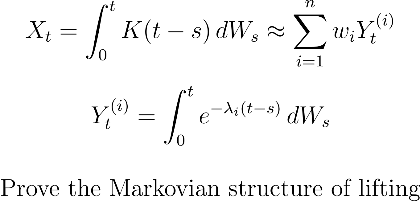
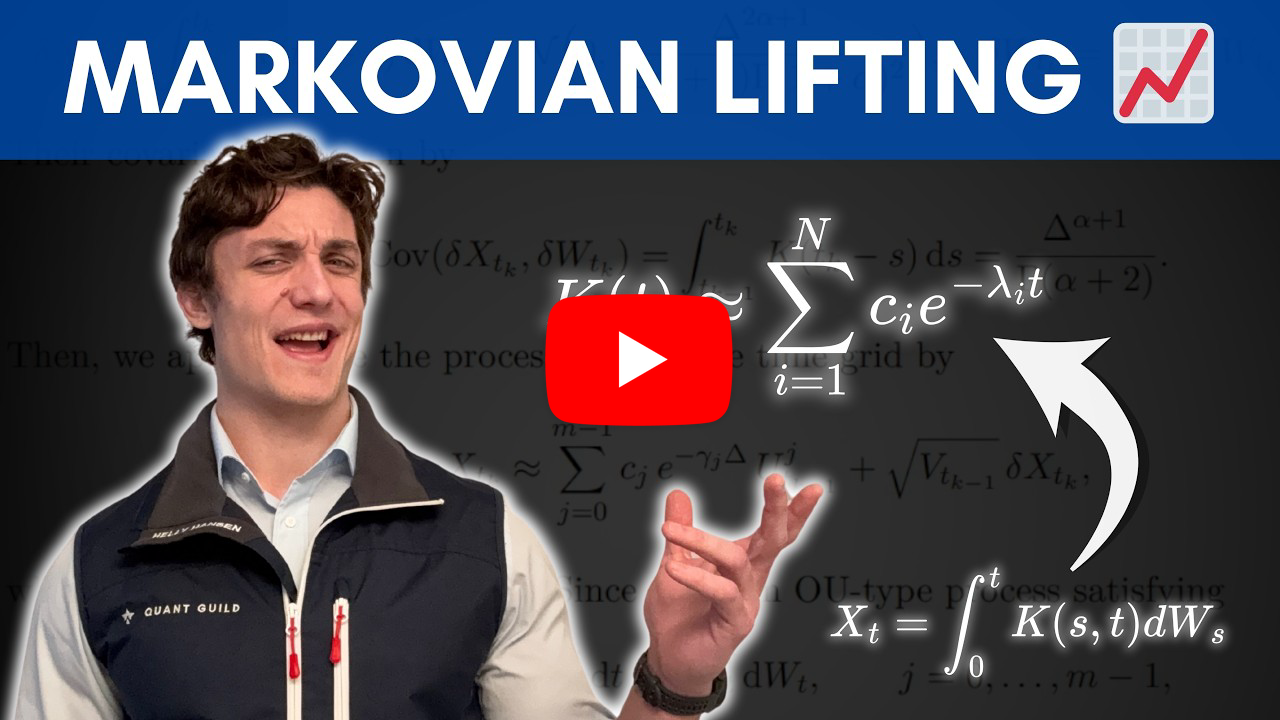
📈 Stop Using the Sharpe Ratio Until You Watch This | In this video I explain why the Sharpe ratio is one of the most misunderstood metrics in trading and why relying on it alone can be dangerous. Most people think it measures return per unit of risk, but in reality it is just a compression of information from a single realized path. It does not tell you how that path was generated, and it cannot distinguish between strategies that look identical statistically but behave very differently in practice. I start by showing that expected return and variance are properties of a realized path, not guarantees of future behavior. There are infinitely many ways to produce the same statistics, which means you cannot recover the underlying process from them. The Sharpe ratio compresses this information even further, making it impossible to understand the true structure or robustness of a strategy from a single number. I then highlight two major limitations. First, from a geometric perspective, the Sharpe ratio penalizes upside and downside volatility equally. This can lead to situations where a strategy with higher returns appears worse simply because it has more positive variation. Second, and more importantly, it says nothing about forward-looking stability. A high Sharpe ratio is meaningless if the underlying strategy is overfit or based on assumptions that will not hold in live markets. Most performance decay comes from either regime changes or, more commonly, overfitting during backtesting. The purpose of a backtest is not to produce a smooth equity curve, but to find a robust model that generalizes out of sample. Without that, any metric, including Sharpe, is just describing noise. The main takeaway is that the Sharpe ratio is not useless, but it is incomplete. It tells you something about the shape of past performance, but nothing about whether that performance will persist. Real trading is about building robust models and making informed decisions under uncertainty, not optimizing a single metric. Here's a link to the full video 👇 | | | 🎲 How Markovian Lifting Solves the Rough Volatility Problem | In this video I explain how we reconcile one of the biggest tradeoffs in modern quantitative finance. Rough volatility models capture market behavior far better than classical models, but they are inherently non-Markovian and path dependent, which makes them computationally expensive and difficult to work with. The core idea of the video is how we retain those realistic dynamics while recovering efficiency. I start by revisiting the Markov property. In a Markov process, the future depends only on the current state. In rough volatility models, this is no longer true. The next step depends on the entire path, which introduces major computational and analytical challenges. Simply expanding the state space to include the full path does not solve the problem because it removes any efficiency gains. The key insight is Markovian lifting. Instead of tracking the entire path, we approximate the path dependent structure using a finite set of Markovian state variables. This is done by transforming the fractional Volterra kernel into a representation involving a weighted sum of exponential functions. Each of these corresponds to a mean-reverting Ornstein Uhlenbeck process, which is Markovian. By doing this, we effectively replace an infinite dimensional, path dependent system with a finite collection of Markov processes that approximate the same dynamics. This recovers the Markov property, restores affine structure, and dramatically improves computational efficiency. Simulation becomes linear instead of quadratic, and we regain access to tools like fast Fourier methods for pricing and calibration. The main takeaway is that Markovian lifting bridges theory and practice. It allows us to model realistic rough volatility dynamics while keeping the system tractable enough to simulate, calibrate, and use in real trading applications. Here's a link to the full video 👇 | | |
|
|
|---|
|
 | 📈 Why 10,000+ Quants Study on Quant Guild | Quant Guild is the one-stop platform for mastering the math that powers modern finance. With 90+ specialized lessons, adaptive practice with gamified progress that scales with your skill level, real interview questions, courses from A - Z in coding, math, probability & statistics, and exclusive live classes with me, it’s built to take you from fundamentals to the front-office. Everything’s designed for how real quants think and work — focused, practical, and deeply technical. That’s why over 10,000+ students and professionals study on Quant Guild to sharpen their edge and make smarter decisions in the face of uncertainty. | 🏛️ See How Pol Became a Market-Maker with Quant Guild |  |  |
|
|
|---|
| | I'm in QR preparing for technical interviews and your practice helped me brush up on probability, thanks | | |
| | |
|
| | | I learned more here in two days than an entire semester of college | | |
| - Guy on Discord Who DM'd Me |
|
|
|
|---|
|
| | ✅ Quant Question of the Week |
| | | | | | |
|
|
|---|
|

 Roman Paolucci